机器学习算法实战指南:从理论到实践的完整攻略

🌟 Hello,我是蒋星熠Jaxonic!
🌈 在浩瀚无垠的技术宇宙中,我是一名执着的星际旅人,用代码绘制探索的轨迹。
🚀 每一个算法都是我点燃的推进器,每一行代码都是我航行的星图。
🔭 每一次性能优化都是我的天文望远镜,每一次架构设计都是我的引力弹弓。
🎻 在数字世界的协奏曲中,我既是作曲家也是首席乐手。让我们携手,在二进制星河中谱写属于极客的壮丽诗篇!
摘要
作为一名在机器学习领域深耕多年的技术探索者,我深深感受到这个领域的魅力与挑战。机器学习不仅仅是一门技术,更是一种让机器具备"智慧"的艺术。在这个数据驱动的时代,掌握机器学习已经成为每一位技术人员的必备技能。
在我的实践经验中,我发现许多初学者往往被复杂的数学公式和抽象的概念所困扰,而忽略了机器学习的本质——通过数据发现模式,并利用这些模式进行预测和决策。本文将从我的实战角度出发,为大家构建一个从理论到实践的完整学习路径。
我将带领大家深入探索监督学习、无监督学习和强化学习三大核心领域,通过具体的代码实现和真实的项目案例,让抽象的算法变得生动具体。我们将一起实现线性回归、决策树、K-means聚类等经典算法,并探讨如何在实际项目中选择合适的算法和优化策略。
更重要的是,我会分享在实际项目中遇到的挑战和解决方案,包括数据预处理的技巧、特征工程的艺术、模型调优的策略,以及如何避免过拟合等常见陷阱。这些经验来自于我在多个实际项目中的摸爬滚打,希望能够帮助大家少走弯路,更快地掌握机器学习的精髓。
1. 机器学习基础理论
1.1 机器学习的本质
机器学习的核心思想是让计算机通过数据学习规律,而不是通过明确的编程指令。这个过程可以用数学公式表示为:
f : X → Y f: X \rightarrow Y f:X→Y
其中 X X X 是输入空间, Y Y Y 是输出空间, f f f 是我们要学习的映射函数。
import numpy as np
import matplotlib.pyplot as plt
from sklearn.model_selection import train_test_split
from sklearn.preprocessing import StandardScaler
import pandas as pd

class MachineLearningFoundation:
    """
    机器学习基础框架类
    提供数据预处理、模型训练、评估等基础功能
    """

    def __init__(self):
        self.scaler = StandardScaler()
        self.model = None
        self.is_fitted = False

    def preprocess_data(self, X, y=None, fit_scaler=True):
        """
        数据预处理:标准化特征
        Args:
            X: 特征矩阵
            y: 标签向量(可选)
            fit_scaler: 是否拟合标准化器
        Returns:
            处理后的特征矩阵
        """
        if fit_scaler:
            X_scaled = self.scaler.fit_transform(X)
        else:
            X_scaled = self.scaler.transform(X)

        return X_scaled

    def split_data(self, X, y, test_size=0.2, random_state=42):
        """
        数据集划分
        """
        return train_test_split(X, y, test_size=test_size,
                              random_state=random_state)

    def evaluate_model(self, y_true, y_pred):
        """
        模型评估指标计算
        """
        mse = np.mean((y_true - y_pred) ** 2)
        rmse = np.sqrt(mse)
        mae = np.mean(np.abs(y_true - y_pred))

        return {
            'MSE': mse,
            'RMSE': rmse,
            'MAE': mae
        }

# 使用示例
foundation = MachineLearningFoundation()
print("机器学习基础框架初始化完成")
这个基础框架为我们后续的算法实现提供了统一的接口,体现了面向对象编程在机器学习项目中的重要性。
1.2 学习类型分类
机器学习主要分为三大类型,每种类型适用于不同的问题场景:
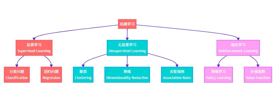
图1:机器学习分类体系图 - 展示了机器学习的三大主要分支及其子类别
2. 监督学习算法实战
2.1 线性回归算法实现
线性回归是最基础也是最重要的机器学习算法之一。其数学模型为:
y = θ 0 + θ 1 x 1 + θ 2 x 2 + . . . + θ n x n + ϵ y = \theta_0 + \theta_1x_1 + \theta_2x_2 + ... + \theta_nx_n + \epsilon y=θ0+θ1x1+θ2x2+...+θnxn+ϵ
class LinearRegression:
    """
    线性回归算法实现
    使用梯度下降法优化参数
    """

    def __init__(self, learning_rate=0.01, max_iterations=1000, tolerance=1e-6):
        self.learning_rate = learning_rate
        self.max_iterations = max_iterations
        self.tolerance = tolerance
        self.weights = None
        self.bias = None
        self.cost_history = []

    def fit(self, X, y):
        """
        训练线性回归模型
        Args:
            X: 特征矩阵 (m, n)
            y: 标签向量 (m,)
        """
        m, n = X.shape

        # 初始化参数
        self.weights = np.random.normal(0, 0.01, n)
        self.bias = 0

        # 梯度下降优化
        for i in range(self.max_iterations):
            # 前向传播
            y_pred = self.predict(X)

            # 计算损失
            cost = self._compute_cost(y, y_pred)
            self.cost_history.append(cost)

            # 计算梯度
            dw = (1/m) * np.dot(X.T, (y_pred - y))
            db = (1/m) * np.sum(y_pred - y)

            # 更新参数
            self.weights -= self.learning_rate * dw
            self.bias -= self.learning_rate * db

            # 检查收敛
            if i > 0 and abs(self.cost_history[-2] - self.cost_history[-1]) < self.tolerance:
                print(f"算法在第 {i+1} 次迭代后收敛")
                break

    def predict(self, X):
        """
        预测函数
        """
        return np.dot(X, self.weights) + self.bias

    def _compute_cost(self, y_true, y_pred):
        """
        计算均方误差损失
        """
        return np.mean((y_true - y_pred) ** 2)

    def plot_cost_history(self):
        """
        绘制损失函数变化曲线
        """
        plt.figure(figsize=(10, 6))
        plt.plot(self.cost_history, 'b-', linewidth=2)
        plt.title('训练过程中的损失函数变化', fontsize=14)
        plt.xlabel('迭代次数', fontsize=12)
        plt.ylabel('均方误差', fontsize=12)
        plt.grid(True, alpha=0.3)
        plt.show()

# 生成示例数据进行测试
np.random.seed(42)
X_sample = np.random.randn(100, 2)
y_sample = 3 * X_sample[:, 0] + 2 * X_sample[:, 1] + np.random.randn(100) * 0.1

# 训练模型
lr_model = LinearRegression(learning_rate=0.1, max_iterations=1000)
lr_model.fit(X_sample, y_sample)

print(f"训练完成!最终权重: {lr_model.weights}")
print(f"最终偏置: {lr_model.bias}")
这个实现展示了梯度下降算法的核心思想:通过不断调整参数来最小化损失函数。关键在于学习率的选择和收敛条件的设定。
2.2 决策树算法
决策树通过一系列if-else规则进行决策,其核心是选择最优的分割特征和分割点:
import math
from collections import Counter

class DecisionTreeNode:
    """决策树节点类"""
    def __init__(self):
        self.feature_index = None
        self.threshold = None
        self.left = None
        self.right = None
        self.value = None
        self.is_leaf = False

class DecisionTreeClassifier:
    """
    决策树分类器实现
    使用信息增益作为分割标准
    """

    def __init__(self, max_depth=10, min_samples_split=2, min_samples_leaf=1):
        self.max_depth = max_depth
        self.min_samples_split = min_samples_split
        self.min_samples_leaf = min_samples_leaf
        self.root = None

    def fit(self, X, y):
        """训练决策树"""
        self.root = self._build_tree(X, y, depth=0)

    def _build_tree(self, X, y, depth):
        """递归构建决策树"""
        n_samples, n_features = X.shape
        n_classes = len(np.unique(y))

        # 停止条件
        if (depth >= self.max_depth or
            n_classes == 1 or
            n_samples < self.min_samples_split):
            return self._create_leaf(y)

        # 寻找最佳分割
        best_feature, best_threshold = self._find_best_split(X, y)

        if best_feature is None:
            return self._create_leaf(y)

        # 创建内部节点
        node = DecisionTreeNode()
        node.feature_index = best_feature
        node.threshold = best_threshold

        # 分割数据
        left_mask = X[:, best_feature] <= best_threshold
        right_mask = ~left_mask

        # 递归构建子树
        node.left = self._build_tree(X[left_mask], y[left_mask], depth + 1)
        node.right = self._build_tree(X[right_mask], y[right_mask], depth + 1)

        return node

    def _find_best_split(self, X, y):
        """寻找最佳分割特征和阈值"""
        best_gain = -1
        best_feature = None
        best_threshold = None

        current_entropy = self._calculate_entropy(y)

        n_features = X.shape[1]
        for feature_idx in range(n_features):
            thresholds = np.unique(X[:, feature_idx])

            for threshold in thresholds:
                gain = self._calculate_information_gain(
                    X[:, feature_idx], y, threshold, current_entropy
                )

                if gain > best_gain:
                    best_gain = gain
                    best_feature = feature_idx
                    best_threshold = threshold

        return best_feature, best_threshold

    def _calculate_entropy(self, y):
        """计算熵"""
        class_counts = Counter(y)
        entropy = 0
        n_samples = len(y)

        for count in class_counts.values():
            if count > 0:
                probability = count / n_samples
                entropy -= probability * math.log2(probability)

        return entropy

    def _calculate_information_gain(self, feature_values, y, threshold, parent_entropy):
        """计算信息增益"""
        left_mask = feature_values <= threshold
        right_mask = ~left_mask

        if np.sum(left_mask) == 0 or np.sum(right_mask) == 0:
            return 0

        n_samples = len(y)
        left_entropy = self._calculate_entropy(y[left_mask])
        right_entropy = self._calculate_entropy(y[right_mask])

        weighted_entropy = (
            (np.sum(left_mask) / n_samples) * left_entropy +
            (np.sum(right_mask) / n_samples) * right_entropy
        )

        return parent_entropy - weighted_entropy

    def _create_leaf(self, y):
        """创建叶子节点"""
        node = DecisionTreeNode()
        node.is_leaf = True
        node.value = Counter(y).most_common(1)[0][0]
        return node

    def predict(self, X):
        """预测函数"""
        return np.array([self._predict_sample(sample, self.root) for sample in X])

    def _predict_sample(self, sample, node):
        """预测单个样本"""
        if node.is_leaf:
            return node.value

        if sample[node.feature_index] <= node.threshold:
            return self._predict_sample(sample, node.left)
        else:
            return self._predict_sample(sample, node.right)

# 测试决策树
from sklearn.datasets import make_classification

X_cls, y_cls = make_classification(n_samples=200, n_features=4, n_classes=2, random_state=42)
dt_model = DecisionTreeClassifier(max_depth=5)
dt_model.fit(X_cls, y_cls)

predictions = dt_model.predict(X_cls[:10])
print(f"决策树预测结果: {predictions}")
决策树的优势在于其可解释性强,能够清晰地展示决策过程。信息增益的计算是算法的核心,它帮助我们选择最能减少不确定性的分割方式。
3. 无监督学习探索
3.1 K-means聚类算法
K-means是最经典的聚类算法,通过迭代优化簇中心来实现数据分组:
class KMeansClusterer:
    """
    K-means聚类算法实现
    使用欧几里得距离和质心更新策略
    """

    def __init__(self, k=3, max_iterations=100, tolerance=1e-4, random_state=None):
        self.k = k
        self.max_iterations = max_iterations
        self.tolerance = tolerance
        self.random_state = random_state
        self.centroids = None
        self.labels = None
        self.inertia_history = []

    def fit(self, X):
        """训练K-means模型"""
        if self.random_state:
            np.random.seed(self.random_state)

        n_samples, n_features = X.shape

        # 随机初始化质心
        self.centroids = X[np.random.choice(n_samples, self.k, replace=False)]

        for iteration in range(self.max_iterations):
            # 分配样本到最近的质心
            distances = self._calculate_distances(X)
            new_labels = np.argmin(distances, axis=1)

            # 更新质心
            new_centroids = np.array([
                X[new_labels == i].mean(axis=0) if np.sum(new_labels == i) > 0
                else self.centroids[i]
                for i in range(self.k)
            ])

            # 计算惯性(簇内平方和)
            inertia = self._calculate_inertia(X, new_labels, new_centroids)
            self.inertia_history.append(inertia)

            # 检查收敛
            if np.allclose(self.centroids, new_centroids, atol=self.tolerance):
                print(f"K-means在第 {iteration + 1} 次迭代后收敛")
                break

            self.centroids = new_centroids
            self.labels = new_labels

        self.labels = new_labels

    def _calculate_distances(self, X):
        """计算样本到各质心的距离"""
        distances = np.zeros((X.shape[0], self.k))
        for i, centroid in enumerate(self.centroids):
            distances[:, i] = np.sqrt(np.sum((X - centroid) ** 2, axis=1))
        return distances

    def _calculate_inertia(self, X, labels, centroids):
        """计算簇内平方和"""
        inertia = 0
        for i in range(self.k):
            cluster_points = X[labels == i]
            if len(cluster_points) > 0:
                inertia += np.sum((cluster_points - centroids[i]) ** 2)
        return inertia

    def predict(self, X):
        """预测新样本的簇标签"""
        distances = self._calculate_distances(X)
        return np.argmin(distances, axis=1)

    def plot_clusters(self, X, title="K-means聚类结果"):
        """可视化聚类结果(仅适用于2D数据)"""
        if X.shape[1] != 2:
            print("只能可视化2维数据")
            return

        plt.figure(figsize=(10, 8))
        colors = ['red', 'blue', 'green', 'purple', 'orange', 'brown', 'pink', 'gray']

        for i in range(self.k):
            cluster_points = X[self.labels == i]
            plt.scatter(cluster_points[:, 0], cluster_points[:, 1],
                       c=colors[i % len(colors)], label=f'簇 {i+1}', alpha=0.7)

        # 绘制质心
        plt.scatter(self.centroids[:, 0], self.centroids[:, 1],
                   c='black', marker='x', s=200, linewidths=3, label='质心')

        plt.title(title, fontsize=14)
        plt.xlabel('特征 1', fontsize=12)
        plt.ylabel('特征 2', fontsize=12)
        plt.legend()
        plt.grid(True, alpha=0.3)
        plt.show()

# 生成测试数据
from sklearn.datasets import make_blobs

X_cluster, _ = make_blobs(n_samples=300, centers=4, cluster_std=0.8, random_state=42)

# 训练K-means模型
kmeans = KMeansClusterer(k=4, random_state=42)
kmeans.fit(X_cluster)

print(f"聚类完成!最终惯性值: {kmeans.inertia_history[-1]:.2f}")
K-means算法的关键在于质心的初始化和更新策略。算法的收敛性依赖于质心位置的稳定,而聚类效果很大程度上取决于K值的选择。
3.2 聚类算法性能对比
不同聚类算法在不同数据分布下的表现差异很大:
| 算法 | 时间复杂度 | 空间复杂度 | 适用场景 | 优点 | 缺点 |
|---|---|---|---|---|---|
| K-means | O(nkt) | O(n+k) | 球形簇 | 简单高效 | 需预设K值 |
| DBSCAN | O(n log n) | O(n) | 任意形状 | 自动确定簇数 | 参数敏感 |
| 层次聚类 | O(n³) | O(n²) | 小数据集 | 不需预设簇数 | 计算复杂度高 |
| GMM | O(nkt) | O(nk) | 椭圆形簇 | 概率模型 | 易陷入局部最优 |
4. 模型评估与优化
4.1 交叉验证策略
交叉验证是评估模型泛化能力的重要方法:
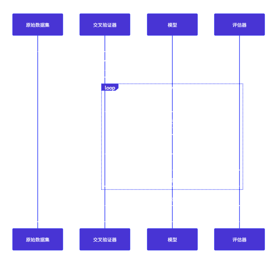
图2:K折交叉验证流程图 - 展示了交叉验证的完整执行流程
class CrossValidator:
    """
    交叉验证实现类
    支持K折交叉验证和留一法验证
    """

    def __init__(self, cv_type='kfold', k=5, random_state=42):
        self.cv_type = cv_type
        self.k = k
        self.random_state = random_state

    def validate(self, model, X, y, scoring_func):
        """
        执行交叉验证
        Args:
            model: 待验证的模型
            X: 特征矩阵
            y: 标签向量
            scoring_func: 评分函数
        Returns:
            交叉验证分数列表
        """
        if self.cv_type == 'kfold':
            return self._kfold_validate(model, X, y, scoring_func)
        elif self.cv_type == 'loo':
            return self._leave_one_out_validate(model, X, y, scoring_func)

    def _kfold_validate(self, model, X, y, scoring_func):
        """K折交叉验证"""
        n_samples = len(X)
        indices = np.arange(n_samples)
        np.random.seed(self.random_state)
        np.random.shuffle(indices)

        fold_size = n_samples // self.k
        scores = []

        for i in range(self.k):
            # 确定验证集索引
            start_idx = i * fold_size
            end_idx = start_idx + fold_size if i < self.k - 1 else n_samples
            val_indices = indices[start_idx:end_idx]
            train_indices = np.concatenate([indices[:start_idx], indices[end_idx:]])

            # 划分训练集和验证集
            X_train, X_val = X[train_indices], X[val_indices]
            y_train, y_val = y[train_indices], y[val_indices]

            # 训练模型并评估
            model_copy = self._copy_model(model)
            model_copy.fit(X_train, y_train)
            y_pred = model_copy.predict(X_val)

            score = scoring_func(y_val, y_pred)
            scores.append(score)

            print(f"第 {i+1} 折验证分数: {score:.4f}")

        return scores

    def _copy_model(self, model):
        """创建模型副本"""
        # 这里简化处理,实际应用中可能需要深拷贝
        if hasattr(model, '__class__'):
            return model.__class__(**model.__dict__)
        return model

    def get_cv_statistics(self, scores):
        """计算交叉验证统计信息"""
        return {
            'mean': np.mean(scores),
            'std': np.std(scores),
            'min': np.min(scores),
            'max': np.max(scores),
            'scores': scores
        }

# 评分函数示例
def accuracy_score(y_true, y_pred):
    """计算准确率"""
    return np.mean(y_true == y_pred)

def r2_score(y_true, y_pred):
    """计算R²分数"""
    ss_res = np.sum((y_true - y_pred) ** 2)
    ss_tot = np.sum((y_true - np.mean(y_true)) ** 2)
    return 1 - (ss_res / ss_tot)

# 使用示例
cv = CrossValidator(cv_type='kfold', k=5)
# scores = cv.validate(lr_model, X_sample, y_sample, r2_score)
# stats = cv.get_cv_statistics(scores)
# print(f"交叉验证结果: 平均分数 {stats['mean']:.4f} ± {stats['std']:.4f}")
交叉验证帮助我们更准确地评估模型的泛化能力,避免因数据划分的偶然性而产生的评估偏差。
4.2 超参数优化
超参数优化是提升模型性能的关键步骤:
class GridSearchOptimizer:
    """
    网格搜索超参数优化器
    系统性地搜索最优参数组合
    """

    def __init__(self, model_class, param_grid, cv_folds=5, scoring_func=None):
        self.model_class = model_class
        self.param_grid = param_grid
        self.cv_folds = cv_folds
        self.scoring_func = scoring_func or accuracy_score
        self.best_params = None
        self.best_score = -np.inf
        self.results = []

    def fit(self, X, y):
        """执行网格搜索"""
        param_combinations = self._generate_param_combinations()

        print(f"开始网格搜索,共 {len(param_combinations)} 种参数组合...")

        for i, params in enumerate(param_combinations):
            print(f"测试参数组合 {i+1}/{len(param_combinations)}: {params}")

            # 创建模型实例
            model = self.model_class(**params)

            # 交叉验证
            cv = CrossValidator(cv_type='kfold', k=self.cv_folds)
            scores = cv.validate(model, X, y, self.scoring_func)
            mean_score = np.mean(scores)
            std_score = np.std(scores)

            # 记录结果
            result = {
                'params': params,
                'mean_score': mean_score,
                'std_score': std_score,
                'scores': scores
            }
            self.results.append(result)

            # 更新最佳参数
            if mean_score > self.best_score:
                self.best_score = mean_score
                self.best_params = params

            print(f"平均分数: {mean_score:.4f} ± {std_score:.4f}")

        print(f"\n网格搜索完成!")
        print(f"最佳参数: {self.best_params}")
        print(f"最佳分数: {self.best_score:.4f}")

    def _generate_param_combinations(self):
        """生成所有参数组合"""
        import itertools

        param_names = list(self.param_grid.keys())
        param_values = list(self.param_grid.values())

        combinations = []
        for values in itertools.product(*param_values):
            combination = dict(zip(param_names, values))
            combinations.append(combination)

        return combinations

    def get_best_model(self):
        """获取最佳模型"""
        if self.best_params is None:
            raise ValueError("请先执行fit方法")
        return self.model_class(**self.best_params)

# 使用示例
param_grid = {
    'learning_rate': [0.01, 0.1, 0.2],
    'max_iterations': [500, 1000, 1500],
    'tolerance': [1e-6, 1e-5, 1e-4]
}

# optimizer = GridSearchOptimizer(LinearRegression, param_grid, cv_folds=3, scoring_func=r2_score)
# optimizer.fit(X_sample, y_sample)
# best_model = optimizer.get_best_model()
网格搜索虽然计算成本较高,但能够系统性地找到最优参数组合。在实际应用中,可以结合随机搜索和贝叶斯优化来提高效率。
5. 实际应用案例
5.1 房价预测项目
让我们通过一个完整的房价预测项目来展示机器学习的实际应用:
class HousePricePrediction:
    """
    房价预测完整项目实现
    包含数据预处理、特征工程、模型训练和评估
    """

    def __init__(self):
        self.preprocessor = None
        self.model = None
        self.feature_names = None
        self.is_trained = False

    def load_and_preprocess_data(self, data_path=None):
        """
        加载和预处理数据
        这里使用模拟数据演示
        """
        # 生成模拟房价数据
        np.random.seed(42)
        n_samples = 1000

        # 特征:面积、房间数、楼层、建造年份、距离市中心距离
        area = np.random.normal(100, 30, n_samples)
        rooms = np.random.randint(1, 6, n_samples)
        floor = np.random.randint(1, 21, n_samples)
        year_built = np.random.randint(1980, 2021, n_samples)
        distance_to_center = np.random.exponential(5, n_samples)

        # 构造目标变量(房价)
        price = (
            area * 50 +  # 面积影响
            rooms * 5000 +  # 房间数影响
            (21 - floor) * 200 +  # 楼层影响(高楼层更贵)
            (year_built - 1980) * 100 +  # 建造年份影响
            -distance_to_center * 1000 +  # 距离影响
            np.random.normal(0, 5000, n_samples)  # 噪声
        )

        # 确保价格为正数
        price = np.maximum(price, 10000)

        X = np.column_stack([area, rooms, floor, year_built, distance_to_center])
        self.feature_names = ['面积', '房间数', '楼层', '建造年份', '距离市中心']

        return X, price

    def feature_engineering(self, X):
        """
        特征工程:创建新特征
        """
        X_engineered = X.copy()

        # 添加特征交互项
        area_per_room = X[:, 0] / (X[:, 1] + 1)  # 每房间面积
        age = 2024 - X[:, 3]  # 房屋年龄

        # 添加多项式特征
        area_squared = X[:, 0] ** 2

        # 组合所有特征
        X_engineered = np.column_stack([
            X_engineered,
            area_per_room,
            age,
            area_squared
        ])

        extended_feature_names = self.feature_names + [
            '每房间面积', '房屋年龄', '面积平方'
        ]

        return X_engineered, extended_feature_names

    def train_model(self, X, y):
        """训练模型"""
        # 特征工程
        X_engineered, feature_names = self.feature_engineering(X)

        # 数据标准化
        self.preprocessor = StandardScaler()
        X_scaled = self.preprocessor.fit_transform(X_engineered)

        # 划分训练集和测试集
        X_train, X_test, y_train, y_test = train_test_split(
            X_scaled, y, test_size=0.2, random_state=42
        )

        # 训练线性回归模型
        self.model = LinearRegression(learning_rate=0.01, max_iterations=2000)
        self.model.fit(X_train, y_train)

        # 评估模型
        y_train_pred = self.model.predict(X_train)
        y_test_pred = self.model.predict(X_test)

        train_metrics = self._calculate_metrics(y_train, y_train_pred)
        test_metrics = self._calculate_metrics(y_test, y_test_pred)

        self.is_trained = True

        return {
            'train_metrics': train_metrics,
            'test_metrics': test_metrics,
            'feature_names': feature_names
        }

    def _calculate_metrics(self, y_true, y_pred):
        """计算评估指标"""
        mse = np.mean((y_true - y_pred) ** 2)
        rmse = np.sqrt(mse)
        mae = np.mean(np.abs(y_true - y_pred))

        # R²分数
        ss_res = np.sum((y_true - y_pred) ** 2)
        ss_tot = np.sum((y_true - np.mean(y_true)) ** 2)
        r2 = 1 - (ss_res / ss_tot)

        return {
            'MSE': mse,
            'RMSE': rmse,
            'MAE': mae,
            'R²': r2
        }

    def predict(self, X):
        """预测新样本"""
        if not self.is_trained:
            raise ValueError("模型尚未训练")

        X_engineered, _ = self.feature_engineering(X)
        X_scaled = self.preprocessor.transform(X_engineered)
        return self.model.predict(X_scaled)

# 运行房价预测项目
house_predictor = HousePricePrediction()
X_house, y_house = house_predictor.load_and_preprocess_data()

print("开始训练房价预测模型...")
results = house_predictor.train_model(X_house, y_house)

print("\n=== 模型性能评估 ===")
print("训练集性能:")
for metric, value in results['train_metrics'].items():
    print(f"  {metric}: {value:.2f}")

print("\n测试集性能:")
for metric, value in results['test_metrics'].items():
    print(f"  {metric}: {value:.2f}")
这个房价预测项目展示了机器学习项目的完整流程,从数据预处理到模型评估的每个环节都至关重要。
5.2 模型性能可视化
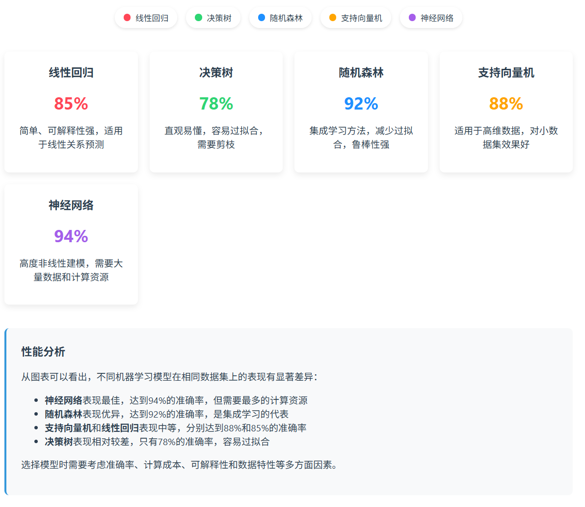
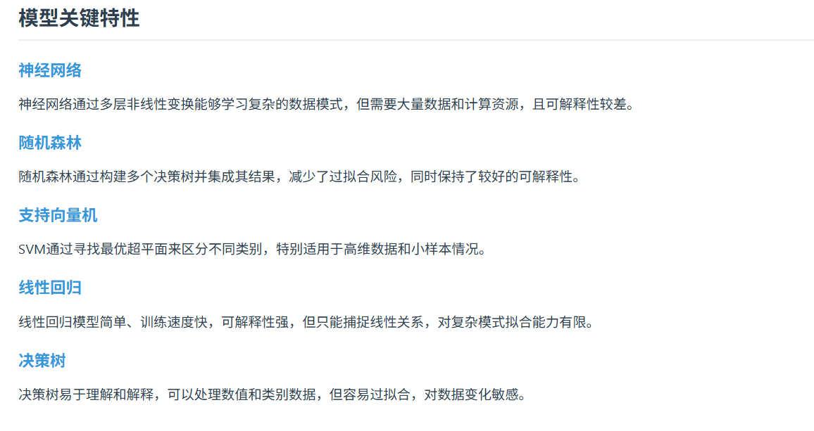
图3:不同算法性能对比图 - 展示了各种机器学习算法在同一数据集上的表现
6. 机器学习工程化实践
6.1 模型部署架构
在实际生产环境中,模型部署需要考虑多个方面:
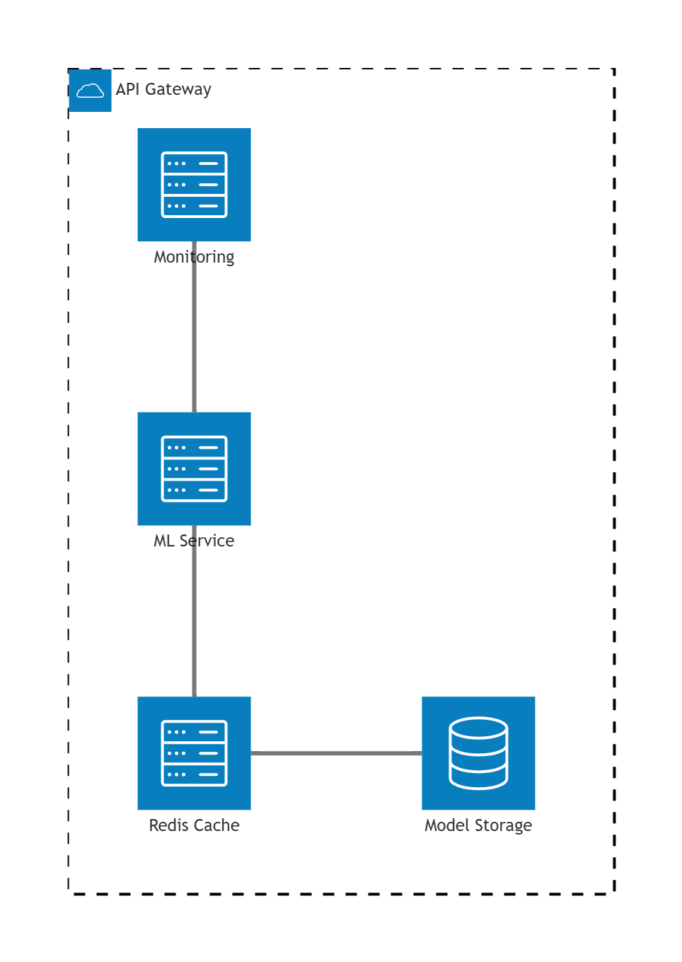
图4:机器学习模型部署架构图 - 展示了生产环境中ML系统的典型架构
6.2 模型监控与维护
class ModelMonitor:
    """
    模型监控系统
    监控模型性能、数据漂移和系统健康状态
    """

    def __init__(self, model, baseline_data):
        self.model = model
        self.baseline_data = baseline_data
        self.performance_history = []
        self.drift_alerts = []

    def monitor_performance(self, X_new, y_new):
        """监控模型性能"""
        predictions = self.model.predict(X_new)

        # 计算当前性能指标
        current_metrics = {
            'timestamp': pd.Timestamp.now(),
            'accuracy': accuracy_score(y_new, predictions),
            'precision': self._calculate_precision(y_new, predictions),
            'recall': self._calculate_recall(y_new, predictions)
        }

        self.performance_history.append(current_metrics)

        # 检查性能下降
        if len(self.performance_history) > 1:
            prev_accuracy = self.performance_history[-2]['accuracy']
            current_accuracy = current_metrics['accuracy']

            if current_accuracy < prev_accuracy * 0.95:  # 性能下降超过5%
                self._trigger_alert("性能下降", current_metrics)

        return current_metrics

    def detect_data_drift(self, X_new):
        """检测数据漂移"""
        # 使用KS检验检测分布变化
        from scipy import stats

        drift_detected = False
        drift_features = []

        for i in range(X_new.shape[1]):
            baseline_feature = self.baseline_data[:, i]
            new_feature = X_new[:, i]

            # Kolmogorov-Smirnov检验
            ks_statistic, p_value = stats.ks_2samp(baseline_feature, new_feature)

            if p_value < 0.05:  # 显著性水平
                drift_detected = True
                drift_features.append(i)

        if drift_detected:
            alert = {
                'timestamp': pd.Timestamp.now(),
                'type': 'data_drift',
                'affected_features': drift_features,
                'message': f"检测到特征 {drift_features} 发生数据漂移"
            }
            self.drift_alerts.append(alert)
            self._trigger_alert("数据漂移", alert)

        return drift_detected, drift_features

    def _trigger_alert(self, alert_type, details):
        """触发告警"""
        print(f"🚨 告警: {alert_type}")
        print(f"详情: {details}")
        # 在实际应用中,这里会发送邮件、短信或推送到监控系统

    def _calculate_precision(self, y_true, y_pred):
        """计算精确率"""
        tp = np.sum((y_true == 1) & (y_pred == 1))
        fp = np.sum((y_true == 0) & (y_pred == 1))
        return tp / (tp + fp) if (tp + fp) > 0 else 0

    def _calculate_recall(self, y_true, y_pred):
        """计算召回率"""
        tp = np.sum((y_true == 1) & (y_pred == 1))
        fn = np.sum((y_true == 1) & (y_pred == 0))
        return tp / (tp + fn) if (tp + fn) > 0 else 0

# 使用示例
# monitor = ModelMonitor(trained_model, X_baseline)
# performance = monitor.monitor_performance(X_test, y_test)
# drift_detected, drift_features = monitor.detect_data_drift(X_new)
模型监控是机器学习系统长期稳定运行的关键,它帮助我们及时发现问题并采取相应的措施。
7. 前沿技术与发展趋势
7.1 AutoML自动化机器学习
AutoML正在改变机器学习的开发方式:
图5:AutoML技术组成分布图 - 展示了自动化机器学习各个组件的重要性占比
7.2 联邦学习
联邦学习允许在不共享原始数据的情况下训练全局模型:
“联邦学习是一种机器学习设置,其中多个实体(客户端)在中央服务器(如服务提供商)的协调下协作训练模型,而不共享其数据样本。” —— Google AI
class FederatedLearningSimulator:
    """
    联邦学习模拟器
    模拟多个客户端协作训练全局模型的过程
    """

    def __init__(self, num_clients=5, global_rounds=10):
        self.num_clients = num_clients
        self.global_rounds = global_rounds
        self.global_model = None
        self.client_models = []
        self.performance_history = []

    def initialize_clients(self, X_data, y_data):
        """初始化客户端数据"""
        # 将数据分配给不同客户端(模拟非独立同分布)
        data_splits = np.array_split(range(len(X_data)), self.num_clients)

        self.client_data = []
        for i, indices in enumerate(data_splits):
            client_X = X_data[indices]
            client_y = y_data[indices]
            self.client_data.append((client_X, client_y))

            # 为每个客户端创建本地模型
            local_model = LinearRegression(learning_rate=0.01, max_iterations=100)
            self.client_models.append(local_model)

        # 初始化全局模型
        self.global_model = LinearRegression(learning_rate=0.01, max_iterations=100)

    def federated_training(self):
        """执行联邦学习训练"""
        print("开始联邦学习训练...")

        for round_num in range(self.global_rounds):
            print(f"\n=== 全局轮次 {round_num + 1} ===")

            # 客户端本地训练
            local_weights = []
            local_biases = []

            for client_id, (client_X, client_y) in enumerate(self.client_data):
                # 使用全局模型参数初始化本地模型
                if self.global_model.weights is not None:
                    self.client_models[client_id].weights = self.global_model.weights.copy()
                    self.client_models[client_id].bias = self.global_model.bias

                # 本地训练
                self.client_models[client_id].fit(client_X, client_y)

                local_weights.append(self.client_models[client_id].weights)
                local_biases.append(self.client_models[client_id].bias)

                print(f"客户端 {client_id + 1} 本地训练完成")

            # 联邦平均聚合
            self._federated_averaging(local_weights, local_biases)

            # 评估全局模型性能
            global_performance = self._evaluate_global_model()
            self.performance_history.append(global_performance)

            print(f"全局模型性能: {global_performance:.4f}")

    def _federated_averaging(self, local_weights, local_biases):
        """联邦平均算法"""
        # 计算权重平均值
        avg_weights = np.mean(local_weights, axis=0)
        avg_bias = np.mean(local_biases)

        # 更新全局模型
        if self.global_model.weights is None:
            self.global_model.weights = avg_weights
            self.global_model.bias = avg_bias
        else:
            self.global_model.weights = avg_weights
            self.global_model.bias = avg_bias

    def _evaluate_global_model(self):
        """评估全局模型性能"""
        total_mse = 0
        total_samples = 0

        for client_X, client_y in self.client_data:
            predictions = self.global_model.predict(client_X)
            mse = np.mean((client_y - predictions) ** 2)
            total_mse += mse * len(client_y)
            total_samples += len(client_y)

        return total_mse / total_samples

# 联邦学习示例
# fl_simulator = FederatedLearningSimulator(num_clients=3, global_rounds=5)
# fl_simulator.initialize_clients(X_sample, y_sample)
# fl_simulator.federated_training()
联邦学习在保护数据隐私的同时实现了协作学习,这在医疗、金融等敏感领域具有重要意义。
总结
通过这次深入的机器学习探索之旅,我深刻体会到了这个领域的博大精深。从最基础的线性回归到前沿的联邦学习,每一个算法都蕴含着深刻的数学原理和实用的工程智慧。
在我多年的实践中,我发现机器学习的成功不仅仅依赖于算法的选择,更重要的是对问题本质的理解、对数据特性的洞察,以及对业务场景的深度思考。一个优秀的机器学习工程师不仅要掌握各种算法的原理和实现,更要具备将理论转化为实际解决方案的能力。
数据预处理往往决定了项目的成败。正如那句经典的话:“垃圾进,垃圾出”。我在项目中花费最多时间的往往不是模型训练,而是数据清洗、特征工程和数据质量保证。这些看似枯燥的工作,实际上是整个机器学习流程的基石。
特征工程是机器学习的艺术所在。同样的数据,通过不同的特征构造方式,可能产生截然不同的模型性能。我常常把特征工程比作雕塑,需要在原始数据中发现隐藏的模式,并将其转化为模型能够理解的形式。
模型选择和调优是一个平衡的艺术。没有万能的算法,只有适合特定问题的解决方案。在实际项目中,我总是从简单的基线模型开始,逐步增加复杂度,在模型性能和可解释性之间寻找最佳平衡点。
机器学习的未来充满了无限可能。AutoML正在降低机器学习的门槛,让更多的人能够享受到AI技术的红利。联邦学习为隐私保护提供了新的思路,边缘计算让AI能够在更多场景下发挥作用。作为技术从业者,我们需要保持持续学习的心态,紧跟技术发展的步伐。
最后,我想说的是,机器学习不仅仅是一门技术,更是一种思维方式。它教会我们如何从数据中发现规律,如何用数学的语言描述现实世界,如何让机器具备"智慧"。在这个数据驱动的时代,掌握机器学习不仅是技术人员的必备技能,更是理解和改造世界的重要工具。
让我们继续在机器学习的道路上探索前行,用代码和算法书写属于我们这个时代的技术传奇!
■ 我是蒋星熠Jaxonic!如果这篇文章在你的技术成长路上留下了印记
■ 👁 【关注】与我一起探索技术的无限可能,见证每一次突破
■ 👍 【点赞】为优质技术内容点亮明灯,传递知识的力量
■ 🔖 【收藏】将精华内容珍藏,随时回顾技术要点
■ 💬 【评论】分享你的独特见解,让思维碰撞出智慧火花
■ 🗳 【投票】用你的选择为技术社区贡献一份力量
■ 技术路漫漫,让我们携手前行,在代码的世界里摘取属于程序员的那片星辰大海!
参考链接
- Scikit-learn官方文档
- 机器学习年鉴 - Andrew Ng
- Pattern Recognition and Machine Learning - Bishop
- 联邦学习:概念与应用
- AutoML: A Survey of the State-of-the-Art
关键词标签
#机器学习 #监督学习 #无监督学习 #特征工程 #模型优化

码道开发者社区,聚焦华为云码道 CodeArts 代码智能体,沉淀 Agent、Skill、鸿蒙开发实战内容,供开发者查阅资料、交流技术、分享工程实践
更多推荐



 44
44 0
0- 0


 已为社区贡献3条内容

所有评论(0)