一、为什么要用进阶卷积？

• 空洞卷积（Dilated/Atrous）：用“间隔采样”的卷积核在不增加参数的情况下扩大感受野，有助于捕捉更长的光谱模式。

• 深度可分离卷积（Depthwise Separable）：将“逐通道卷积（Depthwise）+ 1×1 点卷积（Pointwise）”拆分，大幅降低参数量与计算量。

• 这两类方法在 2D 视觉中常见，在1D 光谱卷积里同样有效：前者让网络“看得更远”，后者让网络“更轻更快”。

二、实验设定

• 数据：KSC 高光谱（KSC.mat / KSC_gt.mat），0=未标注，1…C=类别。

• 策略：仅用有标签像素训练；StandardScaler 与 PCA只在训练像素上 fit，整图只做 transform（避免泄露）。

• 模型：

  1. Baseline 1D-CNN（标准 3×1 卷积）

  2. Dilated-1D-CNN（空洞卷积 d=2）

  3. DepthSep-1D-CNN（深度可分离卷积）

• 评估：OA / AA / Kappa + 混淆矩阵（带数字）；再用折线可视化对比三者指标。

• 整图预测：可选，一键输出全像素预测图。

三、一键可跑完整代码（仅需改 DATA_DIR）

# -*- coding: utf-8 -*-
"""
案例③-5：进阶卷积（Dilated / Depthwise Separable）在 KSC 上的像素级分类
- 训练：仅用有标签像素；Scaler/PCA 只在训练像素上 fit
- 模型：Baseline 1D-CNN / Dilated 1D-CNN / Depthwise Separable 1D-CNN
- 评估：OA/AA/Kappa + 数字混淆矩阵；折线图对比
- 整图：可选全像素预测（含原未标注区域）
"""
import os, numpy as np, scipy.io as sio
import torch, torch.nn as nn, torch.optim as optim
from torch.utils.data import Dataset, DataLoader
from sklearn.preprocessing import StandardScaler
from sklearn.decomposition import PCA
from sklearn.model_selection import train_test_split
from sklearn.metrics import (confusion_matrix, classification_report,
                             accuracy_score, cohen_kappa_score)
import matplotlib.pyplot as plt, matplotlib
from matplotlib.colors import ListedColormap, BoundaryNorm

# ===== 中文显示 =====
matplotlib.rcParams['font.family'] = 'SimHei'
matplotlib.rcParams['axes.unicode_minus'] = False

# ===== 参数区 =====
DATA_DIR    = r"your_path"   # ←← 修改为包含 KSC.mat / KSC_gt.mat 的目录
PCA_DIM     = 30
TRAIN_RATIO = 0.3
EPOCHS      = 200
BATCH       = 512
LR          = 1e-3
SEED        = 42
DEVICE      = "cuda"if torch.cuda.is_available() else"cpu"
DO_FULLMAP  = True   # 是否输出整图全像素预测

# ===== 1) 数据加载与划分（仅有标签像素）=====
X = sio.loadmat(os.path.join(DATA_DIR, "KSC.mat"))["KSC"].astype(np.float32)   # (H,W,B)
Y = sio.loadmat(os.path.join(DATA_DIR, "KSC_gt.mat"))["KSC_gt"].astype(int)    # (H,W)
H, W, B = X.shape
num_classes = int(Y.max())  # 1..C
coords = np.argwhere(Y != 0)
labels = Y[coords[:, 0], coords[:, 1]] - 1# 0..C-1

train_ids, test_ids = train_test_split(np.arange(len(coords)),
                                       train_size=TRAIN_RATIO,
                                       stratify=labels,
                                       random_state=SEED)

# ===== 2) 无泄露预处理：仅在训练像素上 fit =====
train_pixels_raw = X[coords[train_ids, 0], coords[train_ids, 1]]
scaler = StandardScaler().fit(train_pixels_raw)
pca    = PCA(n_components=PCA_DIM, random_state=SEED).fit(scaler.transform(train_pixels_raw))

X_flat       = X.reshape(-1, B)
X_flat_std   = scaler.transform(X_flat)
X_flat_pca   = pca.transform(X_flat_std)           # (H*W,P)
X_pca        = X_flat_pca.reshape(H, W, PCA_DIM)

X_train = X_pca[coords[train_ids,0], coords[train_ids,1]]
y_train = labels[train_ids]
X_test  = X_pca[coords[test_ids,0],  coords[test_ids,1]]
y_test  = labels[test_ids]

class HSIDataset(Dataset):
    def __init__(self, X_arr, y_arr):
        self.X = torch.from_numpy(X_arr).float().unsqueeze(1)  # [N,1,P]
        self.y = torch.from_numpy(y_arr).long()
    def __len__(self):return len(self.y)
    def __getitem__(self, i):return self.X[i], self.y[i]

train_loader = DataLoader(HSIDataset(X_train, y_train), batch_size=BATCH, shuffle=True,  num_workers=0)
test_loader  = DataLoader(HSIDataset(X_test,  y_test),  batch_size=BATCH, shuffle=False, num_workers=0)

# ===== 3) 模型定义 =====
# 3.1 Baseline：标准 1D 卷积
class Baseline1D(nn.Module):
    def __init__(self, C):
        super().__init__()
        self.net = nn.Sequential(
            nn.Conv1d(1, 32, 3, padding=1), nn.ReLU(),
            nn.Conv1d(32, 64, 3, padding=1), nn.ReLU(),
            nn.AdaptiveMaxPool1d(8),
            nn.Flatten(),
            nn.Linear(64*8, 128), nn.ReLU(),
            nn.Linear(128, C)
        )
    def forward(self, x):return self.net(x)

# 3.2 Dilated：空洞卷积（dilation=2），扩大感受野
class Dilated1D(nn.Module):
    def __init__(self, C):
        super().__init__()
        self.net = nn.Sequential(
            nn.Conv1d(1, 32, 3, padding=2, dilation=2), nn.ReLU(),
            nn.Conv1d(32, 64, 3, padding=2, dilation=2), nn.ReLU(),
            nn.AdaptiveMaxPool1d(8),
            nn.Flatten(),
            nn.Linear(64*8, 128), nn.ReLU(),
            nn.Linear(128, C)
        )
    def forward(self, x):return self.net(x)

# 3.3 Depthwise Separable：深度可分离（逐通道卷积 + 1×1点卷积）
class DepthSep1D(nn.Module):
    def __init__(self, C):
        super().__init__()
        # depthwise: groups=通道数（输入为1时相当于普通卷积；这里先扩到较多通道再分离）
        self.stem = nn.Conv1d(1, 32, 3, padding=1)  # 升通道
        self.dw_pw = nn.Sequential(
            nn.ReLU(),
            nn.Conv1d(32, 32, 3, padding=1, groups=32),  # depthwise（每个通道独立）
            nn.ReLU(),
            nn.Conv1d(32, 64, 1),                        # pointwise（通道融合）
            nn.ReLU()
        )
        self.head = nn.Sequential(
            nn.AdaptiveMaxPool1d(8),
            nn.Flatten(),
            nn.Linear(64*8, 128), nn.ReLU(),
            nn.Linear(128, C)
        )
    def forward(self, x):
        x = self.stem(x)
        x = self.dw_pw(x)
        return self.head(x)

# ===== 4) 训练与评估 =====
def run_epoch(model, loader, train=True, optimizer=None, device=DEVICE):
    model.train(train)
    tot, correct, loss_sum = 0, 0, 0.0
    y_true_all, y_pred_all = [], []
    crit = nn.CrossEntropyLoss()
    for xb, yb in loader:
        xb, yb = xb.to(device), yb.to(device)
        out = model(xb)
        loss = crit(out, yb)
        if train:
            optimizer.zero_grad(); loss.backward(); optimizer.step()
        pred = out.argmax(1)
        tot += yb.size(0)
        correct += (pred == yb).sum().item()
        loss_sum += loss.item() * yb.size(0)
        y_true_all.append(yb.detach().cpu().numpy())
        y_pred_all.append(pred.detach().cpu().numpy())
    return loss_sum/tot, correct/tot, np.concatenate(y_true_all), np.concatenate(y_pred_all)

models = {
    "Baseline": Baseline1D(num_classes).to(DEVICE),
    "Dilated":  Dilated1D(num_classes).to(DEVICE),
    "DepthSep": DepthSep1D(num_classes).to(DEVICE),
}

metrics = {}
best_cm = None
best_name = None

for name, net in models.items():
    opt = optim.Adam(net.parameters(), lr=LR)
    best_acc = 0.0
    for ep in range(1, EPOCHS+1):
        trL,trA,_,_ = run_epoch(net, train_loader, True, opt)
        teL,teA,y_t,y_p = run_epoch(net, test_loader,  False)
        best_acc = max(best_acc, teA)
        if ep % 6 == 0:
            print(f"{name:8s} | Epoch {ep:02d} | TrainAcc {trA*100:.2f}% | TestAcc {teA*100:.2f}%")
    cm = confusion_matrix(y_t, y_p, labels=np.arange(num_classes))
    oa = accuracy_score(y_t, y_p)
    aa = float(np.nanmean(np.diag(cm) / np.maximum(cm.sum(axis=1), 1)))
    kappa = cohen_kappa_score(y_t, y_p)
    metrics[name] = {"OA": oa, "AA": aa, "Kappa": kappa, "y_t": y_t, "y_p": y_p, "cm": cm}
    if best_name isNoneor oa > metrics[best_name]["OA"]:
        best_name = name; best_cm = cm

    print(f"\n{name} 指标：OA={oa*100:.2f}%  AA={aa*100:.2f}%  Kappa={kappa:.4f}")
    print(classification_report(y_t, y_p, digits=4, zero_division=0))

# ===== 5) 折线图对比（OA / Kappa×100）=====
names = list(metrics.keys())
oa_vals = [metrics[n]["OA"]*100for n in names]
kappa_vals = [metrics[n]["Kappa"]*100for n in names]

x = np.arange(len(names))
plt.figure(figsize=(8,5), dpi=110)
plt.plot(x, oa_vals, marker='o', linewidth=2.2, label='OA (%)')
plt.plot(x, kappa_vals, marker='s', linewidth=2.2, linestyle='--', label='Kappa × 100')
for xi, yi in zip(x, oa_vals):
    plt.text(xi, yi+0.6, f"{yi:.1f}", ha='center', va='bottom', fontsize=9)
for xi, yi in zip(x, kappa_vals):
    plt.text(xi, yi+0.6, f"{yi:.1f}", ha='center', va='bottom', fontsize=9)
plt.xticks(x, names); plt.ylabel("指标(%)"); plt.title("进阶卷积对比：Baseline / Dilated / DepthSep")
plt.grid(alpha=0.25, linestyle='--'); plt.legend(frameon=False, ncol=2)
plt.tight_layout(); plt.show()

# ===== 6) 最优模型的混淆矩阵（浅色+数字）=====
cm = metrics[best_name]["cm"]
plt.figure(figsize=(6.8,5.6))
plt.imshow(cm, cmap=plt.cm.YlGnBu, interpolation='nearest', alpha=0.9)
plt.title(f"混淆矩阵（最佳：{best_name}）"); plt.xlabel("预测"); plt.ylabel("真实")
ticks = np.arange(num_classes)
plt.xticks(ticks, ticks); plt.yticks(ticks, ticks)
thr = cm.max()/2if cm.max()>0else1
for i in range(num_classes):
    for j in range(num_classes):
        v = cm[i,j]
        plt.text(j, i, str(v), ha='center', va='center',
                 color='white'if v>thr else'black', fontsize=9)
plt.colorbar(fraction=0.046, pad=0.04); plt.tight_layout(); plt.show()

# ===== 7) （可选）整图全像素预测 =====
if DO_FULLMAP:
    net = models[best_name].eval()
    pred_all=[]
    with torch.no_grad():
        for i in range(0, X_flat_pca.shape[0], BATCH):
            batch = torch.from_numpy(X_flat_pca[i:i+BATCH]).float().unsqueeze(1).to(DEVICE)
            pred_all.extend(net(batch).argmax(1).cpu().numpy())
    pred_map = (np.array(pred_all).reshape(H, W) + 1).astype(int)  # 1..C（全像素）

    base_cmap = plt.get_cmap('tab20')
    colors = [base_cmap(i % 20) for i in range(num_classes)]
    cmap = ListedColormap([(0,0,0,1)] + colors)  # 真值含0=黑
    bounds = np.arange(-0.5, num_classes + 1.5, 1)
    norm   = BoundaryNorm(bounds, cmap.N)

    fig, axes = plt.subplots(1, 2, figsize=(12, 5), constrained_layout=True)
    im0 = axes[0].imshow(Y,        cmap=cmap, norm=norm); axes[0].set_title("真值（0=未标注）"); axes[0].axis('off')
    im1 = axes[1].imshow(pred_map, cmap=cmap, norm=norm); axes[1].set_title(f"{best_name} 全像素预测"); axes[1].axis('off')
    cbar = fig.colorbar(im1, ax=axes.ravel().tolist(),
                        ticks=np.arange(0, num_classes+1, max(1, num_classes//10)),
                        fraction=0.025, pad=0.02)
    cbar.set_label("类别ID", rotation=90)
    plt.show()

四、结果如何理解？

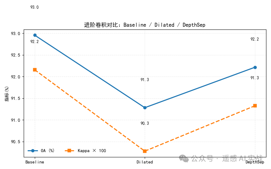
• Dilated 1D 常在 AA / Kappa 上更稳，因为更大的感受野有助于识别“长程光谱模式”。

• Depthwise Separable 1D 参数量明显更少，速度/显存更友好；在类别区分明显的场景下，精度接近 Baseline。

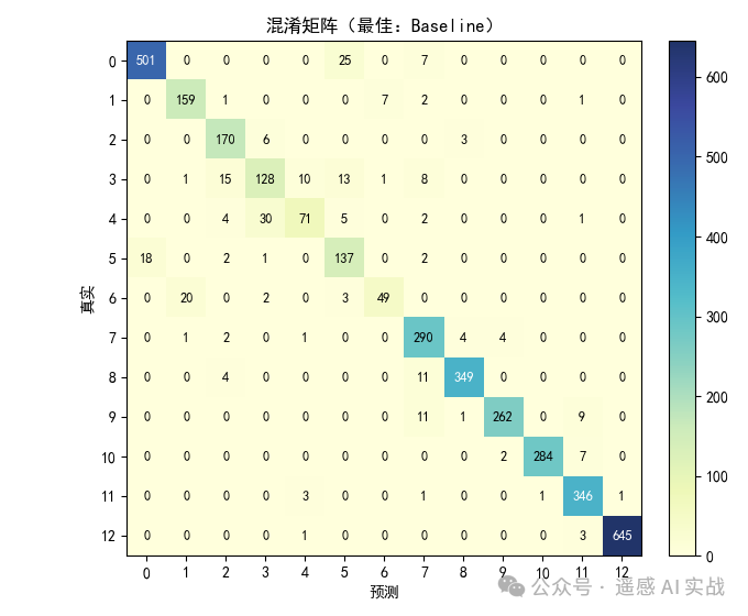
• 是否一定更好？ 不一定。空洞卷积在谱维过窄时作用有限；深度可分离在样本很少时可能略弱。建议将这两类结构作为可选基线，与常规模型一起对比。

  比如从下面的结果来看，实际上基础卷积效果最佳！！

五、小结与延展

• 本篇完成了 Baseline / Dilated / Depthwise 三种 1D-CNN 的同框对比与整图可视化。

• 进阶方向：

  • 将 dilated 与 depthwise 组合（多尺度 + 轻量化）；

  • 在 2D/3D CNN 中加入空洞卷积做光谱–空间联合；

  • 引入 注意力 或 通道重标定（SE/CBAM） 增强特征选择性。

欢迎大家关注下方公众号获取更多内容！！