机器学习入门(2)-KNN,朴素贝叶斯,决策树,随机森林
1、K-近邻算法
案例预测入住位置
- 公式复习:
欧氏距离的计算公式:
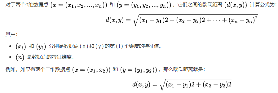
- 分类算法—KNN
定义:如果一个样本在特征空间中的k个最相似(即特征空间中最邻近)的样本中的大多数属于某一个类别,则该样本也属于这个类别
相似的样本,特征之间的值应该是相近的
需要做标准化处理
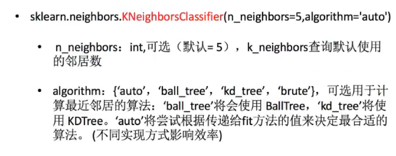
K-近邻算法的API:
- 实例:预测入住位置
官网:(https://www.kaggle.com/navoshta/grid-knn/data)[https://www.kaggle.com/navoshta/grid-knn/data]
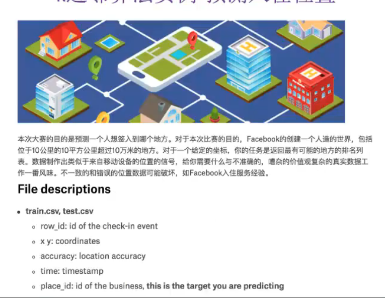
特征值:x,y坐标,定位准确性,时间戳,日,时,周
- 由于数据量大,节省时间x,y缩小
- 时间戳进行(年,月,日,周,时分秒),当作新的特征
- 几千~几万,少于指定签到人数的位置删除
步骤:
- 对于数据做一些基本处理(这里所做的一些处理不一定达到很好的效果,我们只是简单尝试,有些特征我们可以根据一些特征选择的方式去做处理)
- 1 缩小数据集范围 DataFrame.query()
- 2 选取有用的时间特征
- 3 将签到位置少于n个用户的删除
- 分割数据集
- 标准化处理
- k-近邻预测
import pandas as pd
from sklearn.model_selection import train_test_split
from sklearn.neighbors import KNeighborsClassifier
from sklearn.preprocessing import StandardScaler
from sklearn.metrics import accuracy_score

def knncls():
    """
    K-近邻预测用户签到位置
    :return:None
    """
    # 读取数据
    data = pd.read_csv('train.csv')
    test = pd.read_csv('test.csv')
    # 处理数据
    # 1.缩小数据,查询数据筛选
    # x,y刚好返回一个正方形
    data=data.query("x>1.0 & x<1.25 & y>2.5 &y<2.75")
    # 处理时间的数据,将时间戳数据转换为可读的日期时间格式,指定时间戳的单位是秒(seconds)
    time_value=pd.to_datetime(data['time'],unit='s')
    # 把日期转换为字典格式
    time_value=pd.DatetimeIndex(time_value)
    # 构造一些特征
    data['day']=time_value.day
    data['hour']=time_value.hour
    data['weekday']=time_value.weekday
    # 把时间戳特征删除,按列操作
    data=data.drop(['time'],axis=1)
    # 把签到数量少于n个的目标位置删除
    place_count=data.groupby('place_id').count()
    tf=place_count[place_count.row_id>3].reset_index() #reset_index重新索引
    data=data[data['place_id'].isin(tf.place_id)]
    # 删除 row_id 列
    if 'row_id' in data.columns:
        data = data.drop(['row_id'], axis=1)

    # 取出数据当中的特征值和目标值
    x=data.drop(['place_id'],axis=1)
    y=data['place_id']
    # 进行数据的分割,分割成训练集和测试集
    x_train,x_test,y_train,y_test=train_test_split(x,y,test_size=0.25,random_state=42)
    # 特征工程(标准化)
    scaler = StandardScaler()
    x_train = scaler.fit_transform(x_train)
    x_test = scaler.transform(x_test)
    # 进行算法流程
    knn=KNeighborsClassifier(n_neighbors=5)
    knn.fit(x_train,y_train)
    # 得出预测结果
    y_predict=knn.predict(x_test)
    print("预测的目标签到位置为:",y_predict)
    # 得出准确率
    print("预测的准确率:",knn.score(x_test,y_test))

if __name__=="__main__":
    knncls()

输出:
预测的目标签到位置为: [4932578245 5606572086 3992589015 ... 5606572086 6861654717 9710472407]
预测的准确率: 0.48156028368794324
算法总结
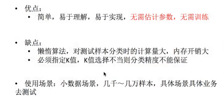
K值取很小:容易受异常点影响
K值取很大,容易受K值数量(类别)波动
fit(X, y)—— 训练(存储数据)
- 作用:把训练集的特征值
X和 目标值y“喂”进模型。 - KNN 的特殊性:
- 它不像逻辑回归、神经网络那样需要学习参数。
fit本质上只是 把训练数据存起来,后续预测时用。- 所以
fit在 KNN 里非常快。
例子:
knn.fit(X_train, y_train)
相当于告诉模型:训练集中这些样本(X_train)对应的类别是这些(y_train)。
predict(X)—— 预测
- 作用:给定新的样本(特征矩阵
X),预测它的类别/输出值。 - 过程:
- 计算该样本与训练集中每个点的距离(通常是欧式距离,也可以设成曼哈顿距离等)。
- 找到最近的
k个邻居。 - 对这
k个邻居的类别进行投票(分类任务)或取平均(回归任务)。 - 输出最终预测值。
例子:
y_pred = knn.predict(X_test)
输出 y_pred,就是测试集中每个样本的预测标签
score(X, y)—— 评估模型
- 作用:计算模型在给定数据上的 评分。
- 在分类问题里:返回 预测准确率(accuracy)。
- 即:
正确预测的样本数 / 总样本数。
- 即:
- 在回归问题里:返回 决定系数 R²。
例子:
acc = knn.score(X_test, y_test)
输出的是一个 0~1 的小数,比如 0.86,表示模型在测试集上的准确率是 86%。
fit(X, y)→ 存训练数据predict(X)→ 用距离 + 投票/平均,得到预测值score(X, y)→ 在给定数据集上计算准确率(分类)或 R²(回归)
2、朴素贝叶斯
主要用于文本分类
算法原理
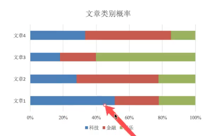
概率是一件事情发生的可能性
- 联合概率:包含多个条件,且所有条件同时成立的概率
- 记作: ( P(A, B) )
( P(A, B) = P(A) P(B) )
- 记作: ( P(A, B) )
- 条件概率:就是事件A在另外一个事件B已经发生条件下的发生概率
- 记作: ( P(A|B) )
- 特性:
( P(A1, A2|B) = P(A1|B) P(A2|B) ) - 注意:此条件概率的成立,是由于A1, A2相互独立的结果
- 基本思想
朴素贝叶斯是一类 基于概率的分类算法,核心是利用 贝叶斯定理 来计算样本属于某一类的概率
“朴素”:也就是条件独立
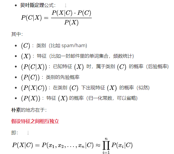
-
拉普拉斯平滑:

-
sklearn朴素贝叶斯实现API
sklearn.naive_bayes.MultinomialNB
sklearn.naive_bayes.MultinomialNB(alpha = 1.0)
- 朴素贝叶斯分类
- alpha:拉普拉斯平滑系数
- 根据公式推导:
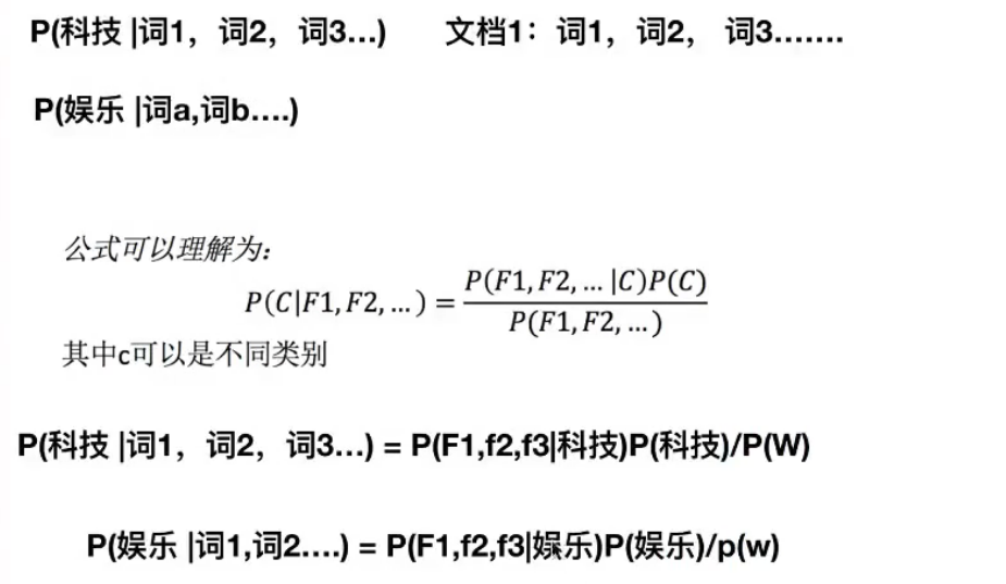
所以,我们只需要求:
P(科技|词1,词2,词3…) = P(F1, f2, f3|科技) P(科技)
P(娱乐|词1,词2…) = P(F1, f2, f3|娱乐) P(娱乐)
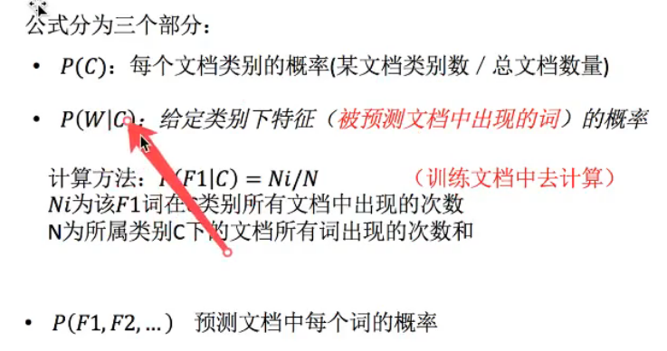
- 举个例子-----预测文档:
训练集有很多个文档,训练集统计结果(指定统计词频):
| 特征统计 | 科技(30篇) | 娱乐(60篇) | 汇总(90篇) |
|---|---|---|---|
| “商场” | 9 | 51 | 60 |
| “影院” | 8 | 56 | 64 |
| “支付宝” | 20 | 15 | 35 |
| “云计算” | 63 | 0 | 63 |
| 汇总(求和) | 100 | 121 | 221 |
现在有一篇被预测文档:出现了影院、支付宝、云计算,计算属于科技、娱乐的类别概率?
解题思路:
求:
- P(科技|影院,支付宝,云计算) = P(影院,支付宝,云计算|科技) P(科技)
- P(娱乐|影院,支付宝,云计算) = P(影院,支付宝,云计算|娱乐) P(娱乐)
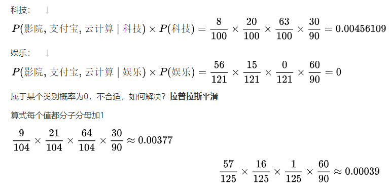
所以为科技类
对新闻进行分类案例
sklearn 20类新闻分类
20个新闻组数据集包含20个主题的18000个新闻组帖子
流程:
- 加载20类新闻数据,并进行分割
- 生成文字特征词
- 朴素贝叶斯estimator流程进行评估
from sklearn.datasets import fetch_20newsgroups
from sklearn.feature_extraction.text import TfidfVectorizer
from sklearn.naive_bayes import MultinomialNB
from sklearn.model_selection import train_test_split
def naviebayes():
    """
    朴素贝叶斯进行文本分类
    :return:None
    """
    news=fetch_20newsgroups(subset="all")
    # 进行数据分割
    x_train,x_test,y_train,y_test=train_test_split(news.data,news.target,test_size=0.25)
    # 对数据集进行特征抽取(TF-IDF)
    tf=TfidfVectorizer()
    # 以训练集当中的词的列表进行每篇文章重要性统计['a','b','c','d']
    x_train=tf.fit_transform(x_train)
    print(tf.get_feature_names_out())
    x_test=tf.transform(x_test)
    # 朴素贝叶斯算法的预测
    mlt=MultinomialNB(alpha=1.0)
    # 打印训练集
    print(x_train)
    mlt.fit(x_train,y_train)
    y_predict=mlt.predict(x_test)
    print("预测的文章类别为:",y_predict)
    # 得出准确率
    print("准确率为:",mlt.score(x_test,y_test))
    return None
if __name__=="__main__":
    naviebayes()
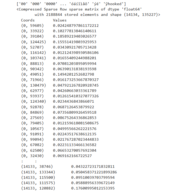
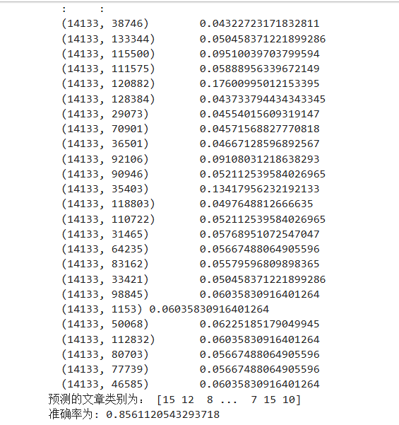
这个没什么超参数可以改,无需调参,所以准确率不好提高,结果基本取决于你的训练集
所以训练集误差大会严重影响结果
算法总结
优点:
- 朴素贝叶斯模型发源于古典数学理论,有稳定的分类效率。
- 对缺失数据不太敏感,算法也比较简单,常用于文本分类。
- 分类准确度高,速度快
缺点:
- 由于使用了样本属性独立性的假设,所以如果样本属性有关联时其效果不好
3、精确率和召回率
分类模型的评估------混淆矩阵
对于二分类问题
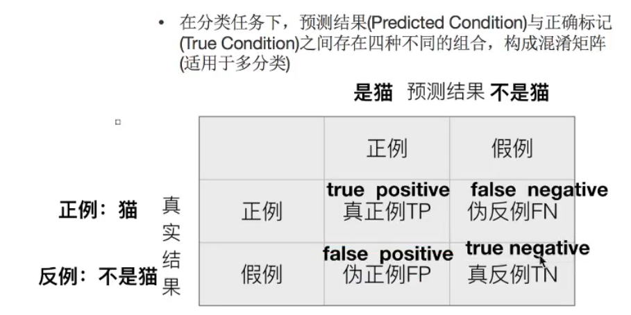
用什么指标去评判?
- 准确率
estimator.score()
- 一般最常见使用的是准确率,即预测结果正确的百分比
- 精确率(Precision)和召回率(Recall)
| 对比维度 | 准确率 (Accuracy) | 精确率 (Precision) |
|---|---|---|
| 计算范围 | 所有样本 | 预测为正的样本 |
| 衡量角度 | 整体正确率 | 正类预测的“纯度” |
| 典型应用 | 样本均衡问题(如图像分类) | 样本不均衡问题(如疾病检测、垃圾邮件) |
| 误报/漏报权重 | 一视同仁 | 更关注“误报”问题 |
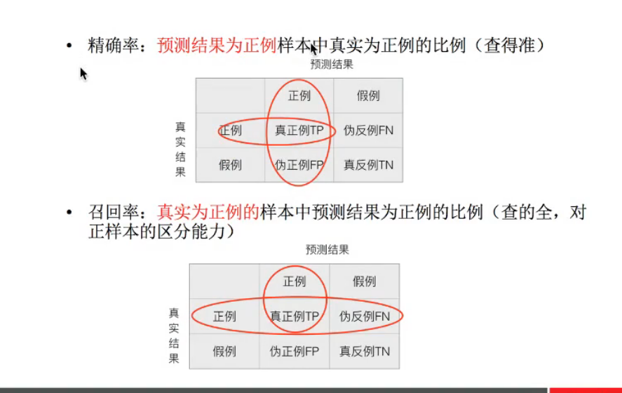
精确率和召回率的API:sklearn.metrics.classification_report
- sklearn.metrics.classification_report(y_true, y_pred, target_names=None)
- y_true: 真实目标值
- y_pred: 估计器预测目标值
- target_names: 目标类别名称
- return: 每个类别精确率与召回率
from sklearn.metrics import classification_report
from sklearn.datasets import fetch_20newsgroups
from sklearn.feature_extraction.text import TfidfVectorizer
from sklearn.naive_bayes import MultinomialNB
from sklearn.model_selection import train_test_split
def naviebayes():
    """
    朴素贝叶斯进行文本分类
    :return:None
    """
    news=fetch_20newsgroups(subset="all")
    # 进行数据分割
    x_train,x_test,y_train,y_test=train_test_split(news.data,news.target,test_size=0.25)
    # 对数据集进行特征抽取(TF-IDF)
    tf=TfidfVectorizer()
    # 以训练集当中的词的列表进行每篇文章重要性统计['a','b','c','d']
    x_train=tf.fit_transform(x_train)
    print(tf.get_feature_names_out())
    x_test=tf.transform(x_test)
    # 朴素贝叶斯算法的预测
    mlt=MultinomialNB(alpha=1.0)
    # 打印训练集
    print(x_train)
    mlt.fit(x_train,y_train)
    y_predict=mlt.predict(x_test)
    print("预测的文章类别为:",y_predict)
    # 得出准确率
    print("准确率为:",mlt.score(x_test,y_test))
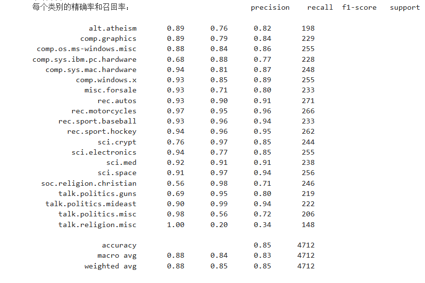
    # 输出朴素贝叶斯模型在每个类别上的分类表现,包括每个类别的精确率(Precision)、召回率(Recall)、F1-score以及样本数量(Support)
    # 打印出朴素贝叶斯分类器在不同类别上的分类性能指标(精确率、召回率、F1 值和样本数)
    print("每个类别的精确率和召回率:",classification_report(y_test,y_predict,target_names=news.target_names))
    return None
if __name__=="__main__":
    naviebayes()
4、交叉验证与网络搜索对K-近邻算法调优
交叉验证
目的:为了让被评估的模型更加准确可信
分为训练集和验证集,得出一个准确率
把数据集平均分成 K 份(folds):
- 每次选其中 1 份作为验证集(validation set)
- 其余 K-1 份作为训练集
- 重复 K 次实验,每次换一份作为验证集
- 最后取 K 次验证结果的平均值,作为模型整体性能指标
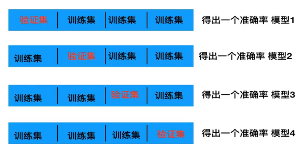
图示为4折交叉验证
网络搜索
就是调参数,比如K-近邻
很多情况下,有很多参数是需要手动指定的(比如K-近邻算法中的k值),这种叫超参数。但是手动过程繁杂,所以需要对模型预设几种超参数组合。每组超参数都采用交叉验证来进行评估。最后选出最优参数组合建立模型

假设有a[2,3,5,8,10],b[20,70,80]两组超参数,那就 每个 a 的值和每个 b 的值配对
| 序号 | a | b |
|---|---|---|
| 1 | 2 | 20 |
| 2 | 2 | 70 |
| 3 | 2 | 80 |
| 4 | 3 | 20 |
| 5 | 3 | 70 |
| 6 | 3 | 80 |
| 7 | 5 | 20 |
| 8 | 5 | 70 |
| 9 | 5 | 80 |
| 10 | 8 | 20 |
| 11 | 8 | 70 |
| 12 | 8 | 80 |
| 13 | 10 | 20 |
| 14 | 10 | 70 |
| 15 | 10 | 80 |
共15组组合
网络搜索的API:sklearn.model_selection.GridSearchCV
sklearn.model_selection.GridSearchCV(estimator, param_grid=None, cv=None)
- 对估计器的指定参数值进行详尽搜索
- estimator:估计器对象
- param_grid:估计器参数(dict){“n_neighbors”:[1,3,5]}
- cv:指定几折交叉验证
- fit:输入训练数据
- score:准确率
结果分析:
- best_score_:在交叉验证中验证的最好结果
- best_estimator_:最好的参数模型
- cv_results_:每次交叉验证后的测试集准确率结果和训练集准确率结果
from sklearn.model_selection import train_test_split,GridSearchCV
import pandas as pd
from sklearn.neighbors import KNeighborsClassifier
from sklearn.preprocessing import StandardScaler
from sklearn.metrics import accuracy_score

def knncls():
    """
    K-近邻预测用户签到位置
    :return:None
    """
    # 读取数据
    data = pd.read_csv('train.csv')
    test = pd.read_csv('test.csv')
    # 处理数据
    # 1.缩小数据,查询数据筛选
    # x,y刚好返回一个正方形
    data=data.query("x>1.0 & x<1.25 & y>2.5 &y<2.75")
    # 处理时间的数据,将时间戳数据转换为可读的日期时间格式,指定时间戳的单位是秒(seconds)
    time_value=pd.to_datetime(data['time'],unit='s')
    # 把日期转换为字典格式
    time_value=pd.DatetimeIndex(time_value)
    # 构造一些特征
    data['day']=time_value.day
    data['hour']=time_value.hour
    data['weekday']=time_value.weekday
    # 把时间戳特征删除,按列操作
    data=data.drop(['time'],axis=1)
    # 把签到数量少于n个的目标位置删除
    place_count=data.groupby('place_id').count()
    tf=place_count[place_count.row_id>3].reset_index() #reset_index重新索引
    data=data[data['place_id'].isin(tf.place_id)]
    # 删除 row_id 列
    if 'row_id' in data.columns:
        data = data.drop(['row_id'], axis=1)

    # 取出数据当中的特征值和目标值
    x=data.drop(['place_id'],axis=1)
    y=data['place_id']
    # 进行数据的分割,分割成训练集和测试集
    x_train,x_test,y_train,y_test=train_test_split(x,y,test_size=0.25,random_state=42)
    # 特征工程(标准化)
    scaler = StandardScaler()
    x_train = scaler.fit_transform(x_train)
    x_test = scaler.transform(x_test)
    # 进行算法流程----超参数
    # 这里的Knn就是网络搜索的实例
    knn=KNeighborsClassifier()
    # 进行网络搜索
    # 构造一些参数的值进行索索
    param={"n_neighbors":[3,5,10]}
    gc=GridSearchCV(knn,param_grid=param,cv=2)  #设置两次交叉验证
    gc.fit(x_train,y_train)
    # 预测准确率
    gc.score(x_test,y_test)
    print("在测试集上的准确率:",gc.score(x_test,y_test))
    print("在交叉验证中最好的结果:",gc.best_score_)
    print("选择最好的模型是:",gc.best_estimator_)
    print("每个超参数每次交叉验证的结果:",gc.cv_results_)
    return None

if __name__=="__main__":
    knncls()


5、决策树
信息论基础
决策树 是一种通过“树形结构”来进行决策的模型。它像人类做决策的思考过程一样:“如果……则……(if…then…)” 一层层判断,直到得出结论
决策树:是一种树形结构,其中每个内部节点表示一个属性上的判断,每个分支代表一个判断结果的输出,最后每个叶节点代表一种分类结果,本质是一颗由多个判断节点组成的树。
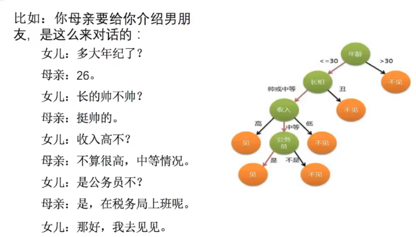
举个例子:
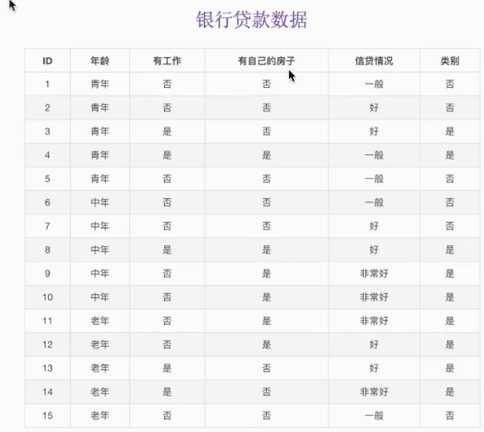
判断你能不能贷款,通过年龄,是否有工作,是否有自己的房子,信贷情况最后得出你你能否贷款
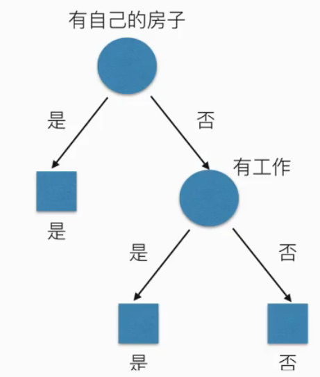
信息熵越大,不确定性越大。像图示所示的树,越往下确认的已知条件越多,确定性越大
划分以及案例
分类依据之一----信息增益
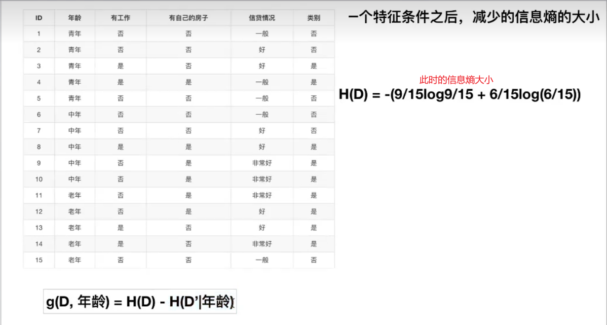
得到一个特征条件之后,减少的信息熵大小
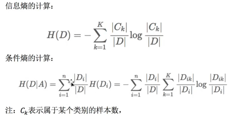
特征A对训练数据集D的信息增益g(D,A),定义为集合D的信息熵H(D)与特征A给定条件下D的信息条件熵H(D|A)之差,即公式为:

注:信息增益表示得知特征X的信息而使得类Y的信息的不确定性减少的程度
| 情况 | 类别比例 | 信息熵H(D) | 意义 |
|---|---|---|---|
| 完全一致(纯净) | (1,0) | 0 | 没有不确定性 |
| 一半一半 | (0.5,0.5) | 1 | 最混乱 |
| 当前情况 | (0.6,0.4) | 0.97 | 仍然较混乱 |
此时信息熵H(D)算出来等于0.97,所以还是比较混乱
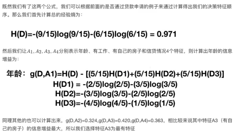
由例子可知,决策树的构建是一个递归划分数据的过程:
- 从数据集中选择一个最优特征作为划分点;
- 按该特征的取值将数据划分成子集;
- 对每个子集重复上述过程;
- 直到满足停止条件(如纯度足够高或树的深度限制)
决策树常用算法
- ID3
信息增益 最大的准则 - C4.5
信息增益比 最大的准则 - CART(划分更加仔细)
回归树:平方误差 最小
分类树:基尼系数 最小的准则 在 sklearn 中可以选择划分的原则
算法API:sklearn.tree.DecisionTreeClassifier
- class sklearn.tree.DecisionTreeClassifier(criterion=‘gini’, max_depth=None, random_state=None)
- 决策树分类器
- criterion:默认为‘gini’系数,也可以选择信息增益的‘entropy’
- max_depth:树的深度大小
- random_state:随机数种子
- method:
- decision_path:返回决策树的路径
案例—泰坦尼克号
- 信息熵和gini系数的对比
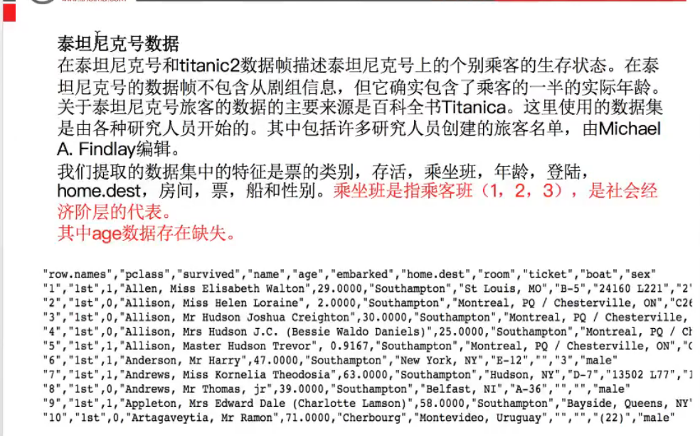
- 1.pd读取数据
- 2.数据基本处理
- 2.1 确定特征值,目标值
- 2.2 缺失值处理
- 2.3 数据集划分
- 3.特征工程(字典特征抽取)
- 4.机器学习(决策树)
- 5.模型评估
import pandas as pd
from sklearn.feature_extraction import DictVectorizer
from sklearn.model_selection import train_test_split
from sklearn.tree import DecisionTreeClassifier
from sklearn.metrics import classification_report, accuracy_score

def decision():
    """
    决策树对泰坦尼克号进行生死预测(将 pclass 也视为类别特征并 one-hot)
    """
    # 1) 读取数据
    titan = pd.read_csv("titanic3.csv")

    # 2) 选择特征与标签
    x = titan[['pclass', 'age', 'sex']].copy()
    y = titan['survived']

    # 3) 缺失值处理
    x['age'] = x['age'].fillna(x['age'].mean())

    # 4) 将 pclass 当作分类特征(转为字符串或 category 都行)
    x['pclass'] = x['pclass'].astype('category')  # 或者 .astype(str)

    # 5) 切分数据
    x_train, x_test, y_train, y_test = train_test_split(
        x, y, test_size=0.25, random_state=42, stratify=y
    )

    # 6) One-hot:DictVectorizer(会对字符串/分类列做 one-hot,对数值列保持原样)
    vec = DictVectorizer(sparse=False)
    x_train_enc = vec.fit_transform(x_train.to_dict(orient="records"))
    x_test_enc  = vec.transform(x_test.to_dict(orient="records"))

    # 看看最终特征名(应包含 pclass=1/2/3 与 sex=female/male)
    feature_names = vec.get_feature_names_out()
    print("特征名:", feature_names)

    # 7) 决策树训练与评估
    # 此处用的信息熵,可以改为gini
    clf = DecisionTreeClassifier(criterion="entropy", max_depth=5, random_state=42)
    clf.fit(x_train_enc, y_train)
    y_pred = clf.predict(x_test_enc)

    print("Accuracy:", accuracy_score(y_test, y_pred))
    print(classification_report(y_test, y_pred))

    # 8)(可选)特征重要性
    importances = pd.Series(clf.feature_importances_, index=feature_names).sort_values(ascending=False)
    print("特征重要性:")
    print(importances)

if __name__ == "__main__":
    decision()
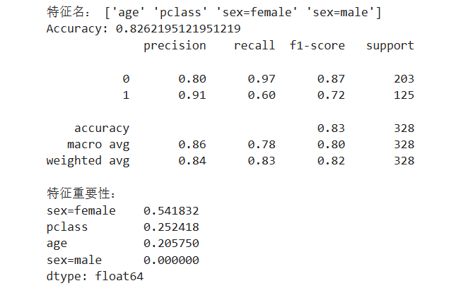
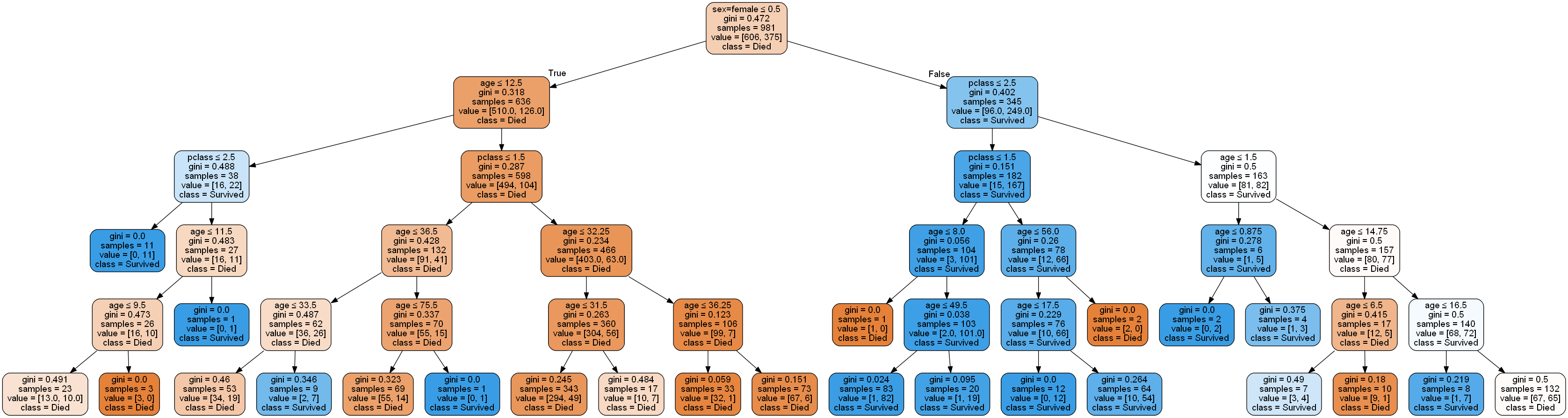
这是使用信息熵的结果:
这是使用基尼系数的结果:
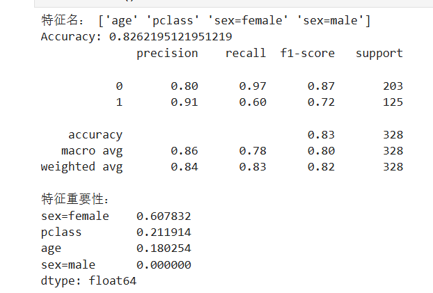
在大多数任务中,Gini 和 Entropy 得到的结果非常接近,差异仅在特征划分的细微偏好
| 对比项 | Entropy | Gini |
|---|---|---|
| 理论来源 | 信息论(ID3 / C4.5) | CART 算法 |
| 计算速度 | 略慢(有 log) | 更快(平方) |
| 结果差异 | 几乎相同 | 几乎相同 |
| 特征偏好 | 对小概率类别更敏感 | 对主导类别更敏感 |
| sklearn 默认 | ❌ | ✅(默认使用 Gini) |
- 决策树的结构、本地保存
用graghviz可视化
sklearn.tree.export_graphviz()该函数能够导出 DOT 格式
tree.export_graphviz(estimator, out_file='tree.dot', feature_names=['', ''])- 工具:(能够将 dot 文件转换为 pdf、png)
安装 graphviz
Ubuntu:sudo apt-get install graphviz
Mac:brew install graphviz - 运行命令
然后我们运行这个命令
$ dot -Tpng tree.dot -o tree.png
import pandas as pd
from sklearn.feature_extraction import DictVectorizer
from sklearn.model_selection import train_test_split
from sklearn.tree import DecisionTreeClassifier
from sklearn.metrics import classification_report, accuracy_score
import graphviz
from sklearn.tree import export_graphviz

def decision():
    """
    决策树对泰坦尼克号进行生死预测(将 pclass 也视为类别特征并 one-hot)
    """
    # 1) 读取数据
    titan = pd.read_csv("titanic3.csv")

    # 2) 选择特征与标签
    x = titan[['pclass', 'age', 'sex']].copy()
    y = titan['survived']

    # 3) 缺失值处理
    x['age'] = x['age'].fillna(x['age'].mean())

    # 4) 将 pclass 当作分类特征(转为字符串或 category 都行)
    x['pclass'] = x['pclass'].astype('category')  # 或者 .astype(str)

    # 5) 切分数据
    x_train, x_test, y_train, y_test = train_test_split(
        x, y, test_size=0.25, random_state=42, stratify=y
    )

    # 6) One-hot:DictVectorizer(会对字符串/分类列做 one-hot,对数值列保持原样)
    vec = DictVectorizer(sparse=False)
    x_train_enc = vec.fit_transform(x_train.to_dict(orient="records"))
    x_test_enc  = vec.transform(x_test.to_dict(orient="records"))

    # 看看最终特征名(应包含 pclass=1/2/3 与 sex=female/male)
    feature_names = vec.get_feature_names_out()
    print("特征名:", feature_names)

    # 7) 决策树训练与评估
    clf = DecisionTreeClassifier(criterion="gini", max_depth=5, random_state=42)
    clf.fit(x_train_enc, y_train)
    y_pred = clf.predict(x_test_enc)

    print("Accuracy:", accuracy_score(y_test, y_pred))
    print(classification_report(y_test, y_pred))

    # 8)(可选)特征重要性
    importances = pd.Series(clf.feature_importances_, index=feature_names).sort_values(ascending=False)
    print("特征重要性:")
    print(importances)

    # 9) 导出为 .dot,并渲染为 PNG
    dot_data = export_graphviz(
        clf,
        out_file=None,
        feature_names=feature_names,
        class_names=["Died", "Survived"],
        filled=True, rounded=True, special_characters=True
    )
    # 写入 .dot 文件
    with open("titanic_tree.dot", "w", encoding="utf-8") as f:
        f.write(dot_data)
    print("已保存:titanic_tree.dot")
    # 用 graphviz 在 Jupyter 中直接渲染
    gragh=graphviz.Source(dot_data)
    display(gragh)
    gragh.render(filename="titanic_tree", format="png", cleanup=True)
    print("已保存为 titanic_tree.png 文件")
    return gragh

if __name__ == "__main__":
    decision()
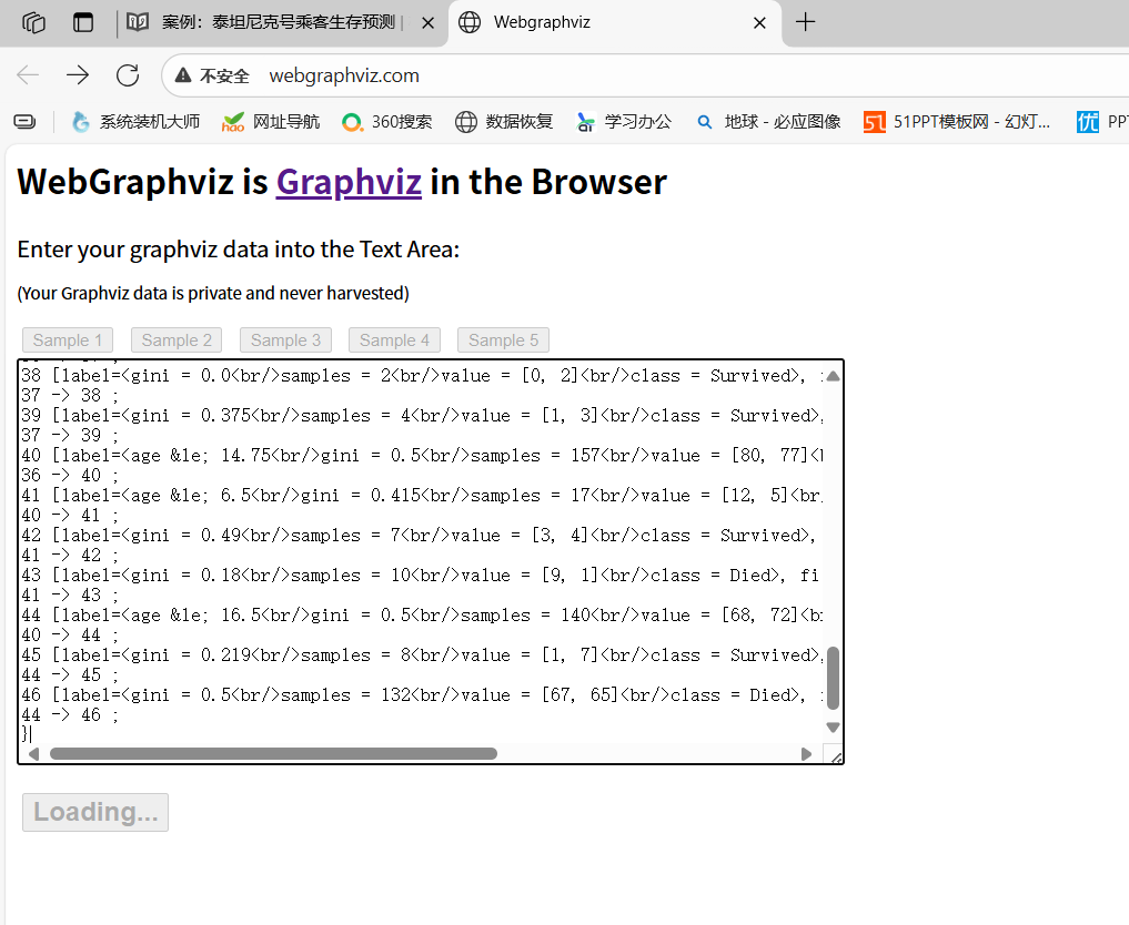
可视化可以把.dot文件内容导入到网址链接上:
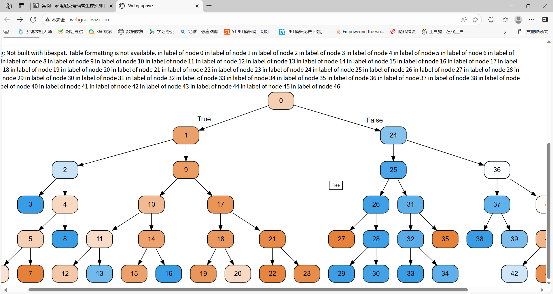
决策树的保存结果分析
决策树优缺点:
优点:
- 简单的理解和解释,决策树可视化。
- 需要很少的数据准备,其他技术通常需要数据归一化。
缺点:
- 决策树学习者可以创建不能很好地推广数据的过于复杂的树,这被称为过拟合。
改进:
- 剪枝cart算法(决策树API当中已经实现,随机森林参数调优有相关介绍)
- 随机森林
注: 企业重要决策,由于决策树很好的分析能力,在决策过程中应用较多。
6、随机森林原理及案例调优
集成学习方法
集成学习通过建立几个模型组合来解决单一预测问题。它的工作原理是生成多个分类器/模型,各自独立地学习和做出预测。这些预测最后结合成单预测,因此优于任何一个单分类的做出预测
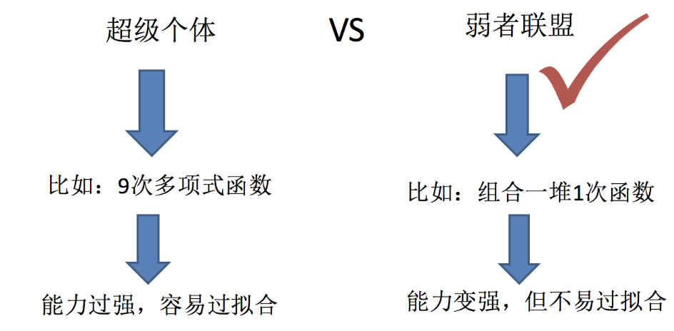
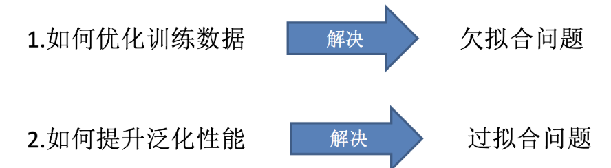
复习—机器学习的2个任务:
什么是随机森林
在机器学习中,随机森林是一个包含了多个决策树的分类器,并且其输出的类别是由个别树输出的类别的众数而定
随机森林 = 多棵决策树 + 随机性 + 投票/平均
例如,如果你训练了5个树,其中有4个树的结果是true,1个数的结果是false,那么最终,结果会是true.
随机森林的过程、优势
- 随机森林建立多个决策树的过程
bootstrap抽样—随机又放回的抽样
原始数据集有 **N 个样本、M 个特征,**我们希望建立 K 棵决策树
一、单棵树的建立过程
步骤 1:随机有放回抽样样本(Bootstrap Sampling)
从原始 N 个样本中,随机抽取 N 个样本(有放回抽样)。
- 意味着:同一个样本可能被抽中多次;
- 大约有 63.2% 的样本会被抽中(称为“袋内样本” in-bag);
- 剩余的约 36.8% 样本没被抽中(称为“袋外样本” out-of-bag,可用于验证)。
这样,每棵树看到的数据都略有不同。
步骤 2:随机选取特征(Feature Subsampling)
在 M 个特征中,随机选取 m 个特征(m ≪ M)供本次树分裂使用。
- 分类问题中,常设 m = √M
- 回归问题中,常设 m = M/3
- 每个节点分裂时都会重新随机选择一组 m 特征。
这一步进一步打破树与树之间的“相似性”,增强模型多样性。
步骤 3:用选出的样本和特征训练一棵决策树
- 使用 CART 算法(基尼指数或最小方差);
- 不剪枝(保持树尽量深);
- 得到一棵弱相关、略有噪声的树。
二、建立多棵树的过程
重复上面 3 个步骤 K 次(通常 K=100~500):
每棵树:
- 用不同的样本子集;
- 用不同的特征子集;
- 独立训练;
- 最后集成到一起形成“森林”。
三、预测阶段
- 分类任务:每棵树投票,取票数最多的类别为最终预测;
- 回归任务:每棵树输出一个值,取平均值作为最终预测。
四、示意总结(结构化表达)
| 步骤 | 内容 | 随机性来源 |
|---|---|---|
| ① 样本抽样 | 从 N 个样本中有放回地抽取 N 个样本 | 样本随机 |
| ② 特征抽样 | 在 M 个特征中随机选择 m 个 | 特征随机 |
| ③ 建树 | 用 CART 算法训练一棵未剪枝的决策树 | 算法过程 |
| ④ 重复 K 次 | 得到 K 棵不同的树 | 集成形成随机森林 |
- 随机森林API
class sklearn.ensemble.RandomForestClassifier(n_estimators=10,criterion=‘gini’,max_depth=None, bootstrap=True, random_state=None)
随机森林分类器
- n_estimators:integer, optional(default = 10) 森林里的树木数量 120, 200, 300, 500, 800, 1000
- criteria:string, 可选(default = “gini”) 分割特征的测量方法
- max_depth:integer 或 None,可选(默认为无) 树的最大深度
5, 8, 15, 25, 30 - max_features = “auto”,每个决策树的最大特征数量
- If “auto”, then
max_features = sqrt(n_features) - If “sqrt”, then
max_features = sqrt(n_features)(same as “auto”) - If “log2”, then
max_features = log2(n_features) - If None, then
max_features = n_features
- If “auto”, then
- bootstrap:boolean, optional(default = True) 是否在构建树时使用有放回抽样
import pandas as pd
from sklearn.feature_extraction import DictVectorizer
from sklearn.model_selection import train_test_split
from sklearn.tree import DecisionTreeClassifier
from sklearn.metrics import classification_report, accuracy_score
from sklearn.ensemble import RandomForestClassifier
from sklearn.model_selection import GridSearchCV

def decision():
    """
    决策树对泰坦尼克号进行生死预测(将 pclass 也视为类别特征并 one-hot)
    """
    # 1) 读取数据
    titan = pd.read_csv("titanic3.csv")

    # 2) 选择特征与标签
    x = titan[['pclass', 'age', 'sex']].copy()
    y = titan['survived']

    # 3) 缺失值处理
    x['age'] = x['age'].fillna(x['age'].mean())

    # 4) 将 pclass 当作分类特征(转为字符串或 category 都行)
    x['pclass'] = x['pclass'].astype('category')  # 或者 .astype(str)

    # 5) 切分数据
    x_train, x_test, y_train, y_test = train_test_split(
        x, y, test_size=0.25, random_state=42, stratify=y
    )

    # 6) One-hot:DictVectorizer(会对字符串/分类列做 one-hot,对数值列保持原样)
    vec = DictVectorizer(sparse=False)
    x_train_enc = vec.fit_transform(x_train.to_dict(orient="records"))
    x_test_enc  = vec.transform(x_test.to_dict(orient="records"))

    # 看看最终特征名(应包含 pclass=1/2/3 与 sex=female/male)
    feature_names = vec.get_feature_names_out()
    print("特征名:", feature_names)

    # 随机森林预测(超参数调优)
    rf=RandomForestClassifier()
    param={"n_estimators":[120,200,300,500,800,1200],"max_depth":[5,8,15,25,30]}
    # 网络搜索与交叉验证
    gc=GridSearchCV(rf,param_grid=param,cv=4)
    gc.fit(x_train_enc, y_train)
    print("准确率为:", gc.score(x_test_enc, y_test))
    print("查看选择的参数模型:",gc.best_params_)
if __name__ == "__main__":
    decision()

输出:
特征名: ['age' 'pclass' 'sex=female' 'sex=male']
准确率为: 0.8170731707317073
查看选择的参数模型: {'max_depth': 5, 'n_estimators': 120}
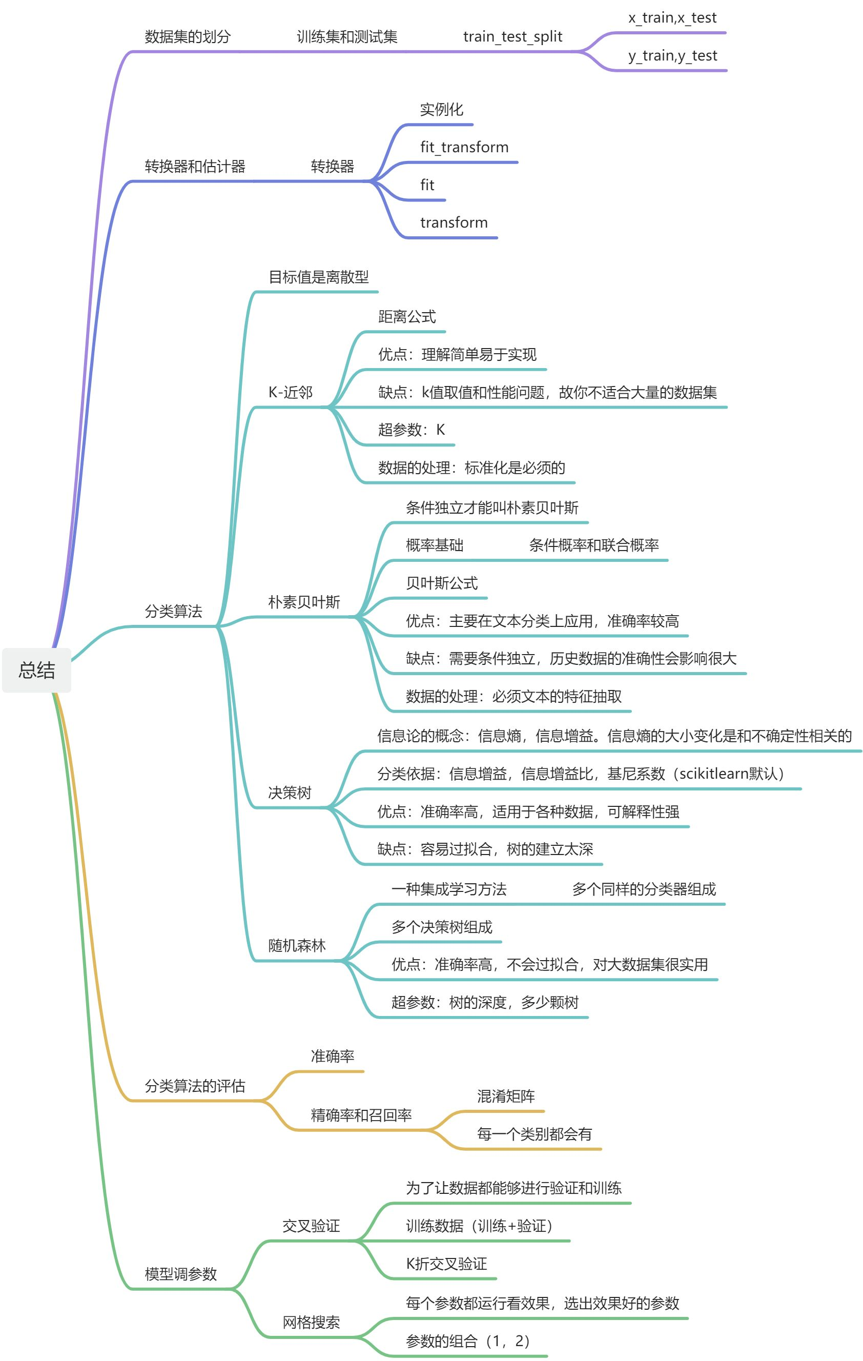
思维导图

码道开发者社区,聚焦华为云码道 CodeArts 代码智能体,沉淀 Agent、Skill、鸿蒙开发实战内容,供开发者查阅资料、交流技术、分享工程实践
更多推荐



 28
28 0
0- 0


 已为社区贡献2条内容

所有评论(0)