【精选优质专栏推荐】

• 《AI 技术前沿》 —— 紧跟 AI 最新趋势与应用
• 《网络安全新手快速入门(附漏洞挖掘案例)》 —— 零基础安全入门必看
• 《BurpSuite 入门教程(附实战图文)》 —— 渗透测试必备工具详解
• 《网安渗透工具使用教程(全)》 —— 一站式工具手册
• 《CTF 新手入门实战教程》 —— 从题目讲解到实战技巧
• 《前后端项目开发(新手必知必会)》 —— 实战驱动快速上手

每个专栏均配有案例与图文讲解，循序渐进，适合新手与进阶学习者，欢迎订阅。

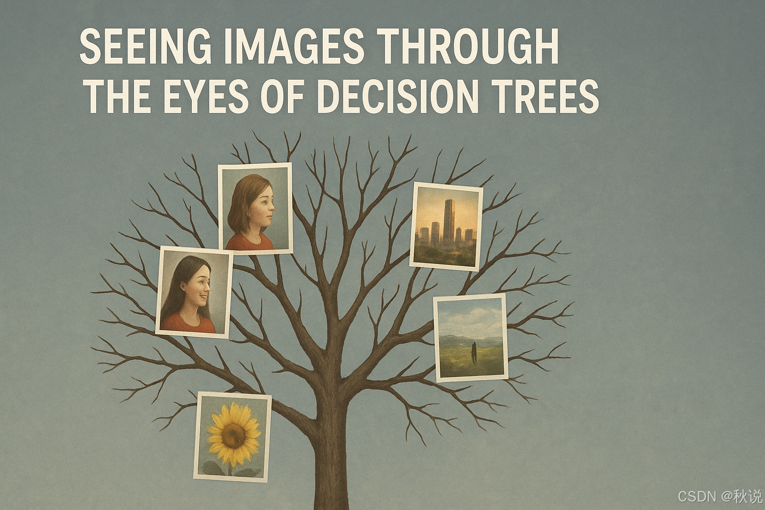
在本文中，你将学习：

• 将非结构化的原始图像数据转化为结构化的、有信息量的特征。
• 基于提取的图像特征训练一个决策树分类器用于图像分类。
• 将上述方法应用到 CIFAR-10 数据集进行图像分类。

引言

众所周知，基于决策树的模型在各种分类和回归任务中表现优异，通常用于结构化的表格数据。但结合合适的工具后，决策树同样可以对非结构化数据（如文本、图像，甚至时间序列数据）发挥强大的预测作用。

本文演示了如何通过将图像数据转化为结构化、有意义的特征，使决策树能够理解图像。具体来说，我们将展示如何把原始的像素级图像数据转化为更高层次的特征，这些特征描述了图像的属性，例如颜色直方图和边缘数量。随后，我们将利用这些信息执行预测任务（如分类），通过训练决策树实现目标——这一切都基于 Python 的 scikit-learn 库。

想象一下：这就像让决策树的“视角”更接近人类眼睛的工作方式。

基于图像特征构建决策树进行图像分类

本教程使用的 CIFAR-10 数据集包含低分辨率的彩色图像（32×32 像素）。每个像素由三个 RGB 值描述，用于定义其颜色。

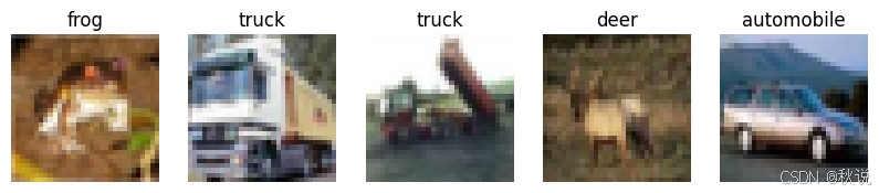
虽然常用的图像分类模型（如神经网络）可以直接处理像素网格，但 决策树 更适合处理结构化数据，因此我们的首要任务是将原始图像数据转换为这种结构化形式。

我们首先加载数据集（TensorFlow 库中可直接获取）：

from tensorflow.keras.datasets import cifar10
import numpy as np
import matplotlib.pyplot as plt

(X_train, y_train), (X_test, y_test) = cifar10.load_data()
y_train = y_train.flatten()
y_test = y_test.flatten()

class_names = ['airplane','automobile','bird','cat','deer',
               'dog','frog','horse','ship','truck']

print("Training set:", X_train.shape, y_train.shape)
print("Test set:", X_test.shape, y_test.shape)

# 可选：显示部分样本
fig, axes = plt.subplots(1, 5, figsize=(10, 3))
for i, ax in enumerate(axes):
    ax.imshow(X_train[i])
    ax.set_title(class_names[y_train[i]])
    ax.axis('off')
plt.show()

注意，加载的数据集已分为训练集和测试集，输出标签（10 个类别）也已与图像数据分开。我们只需使用 Python 元组合理分配即可。为了便于理解，我们还将类别名称保存在列表中。

接下来定义核心函数 extract_features()，用于从图像中提取所需特征。本例中提取两类特征：每个 RGB 通道的颜色直方图，以及图像的边缘强度。

from skimage.color import rgb2gray
from skimage.filters import sobel

def extract_features(images, bins_per_channel=8):
    features = []
    for img in images:
        # RGB 三通道颜色直方图
        hist_features = []
        for c in range(3):
            hist, _ = np.histogram(img[:,:,c], bins=bins_per_channel, range=(0, 255))
            hist_features.extend(hist)

        # 灰度图边缘检测
        gray_img = rgb2gray(img)
        edges = sobel(gray_img)
        edge_strength = np.sum(edges > 0.1)

        # 合并特征
        features.append(hist_features + [edge_strength])
    
    return np.array(features, dtype=np.float32)

每个颜色直方图的分箱数设置为 8，以保持图像颜色信息的密度适中。边缘检测使用 rgb2gray 和 sobel，在原图的灰度版本上提取边缘。两个特征集合合并后，对数据集中的每张图像重复此过程。

然后对训练集和测试集分别调用该函数：

X_train_feats = extract_features(X_train)
X_test_feats = extract_features(X_test)

print("Feature vector size:", X_train_feats.shape[1])

最终，每张图像得到的特征数为 25（RGB 直方图 + 边缘强度）。

完成特征提取后，我们即可训练基于 决策树 的分类器。与直接使用原始像素不同，这里我们将提取后的特征作为输入。

from sklearn.tree import DecisionTreeClassifier
from sklearn.metrics import classification_report, accuracy_score

dt_model = DecisionTreeClassifier(random_state=42, max_depth=20)
dt_model.fit(X_train_feats, y_train)

y_pred_dt = dt_model.predict(X_test_feats)

print("MODEL 1. Decision Tree (Color histograms + Edge count):")
print("Accuracy:", accuracy_score(y_test, y_pred_dt))
print(classification_report(y_test, y_pred_dt, target_names=class_names))

结果示例：

Accuracy: 0.2594
              precision    recall  f1-score   support

    airplane       0.33      0.33      0.33      1000
  automobile       0.30      0.32      0.31      1000
        bird       0.23      0.24      0.24      1000
         cat       0.17      0.18      0.17      1000
        deer       0.24      0.21      0.23      1000
         dog       0.18      0.19      0.19      1000
        frog       0.31      0.31      0.31      1000
       horse       0.22      0.20      0.21      1000
        ship       0.35      0.32      0.33      1000
       truck       0.28      0.30      0.29      1000

    accuracy                           0.26     10000
   macro avg       0.26      0.26      0.26     10000
weighted avg       0.26      0.26      0.26     10000

可以看到，决策树在提取的特征上表现不佳。这完全正常，也在预期之内。

原因在于：将 32×32 的彩色图像压缩为仅 25 个特征，过度简化，丢失了区分鸟和飞机、猫和狗所需的细微信息。同时，同一类别的图像在颜色等属性上差异较大。本文的核心目的不是追求高准确率，而是理解如何为决策树提取图像特征及其局限性。

不过，如果我们使用更复杂的树模型，比如 随机森林分类器，效果会更好吗？

让我们试试：

from sklearn.ensemble import RandomForestClassifier

rf_model = RandomForestClassifier(n_estimators=100, random_state=42, n_jobs=-1)
rf_model.fit(X_train_feats, y_train)

y_pred_rf = rf_model.predict(X_test_feats)

print("MODEL 2. Random Forest (Color histograms + Edge count)")
print("Accuracy:", accuracy_score(y_test, y_pred_rf))
print(classification_report(y_test, y_pred_rf, target_names=class_names))

结果：

Accuracy: 0.3952
              precision    recall  f1-score   support

    airplane       0.49      0.52      0.51      1000
  automobile       0.37      0.48      0.42      1000
        bird       0.36      0.30      0.33      1000
         cat       0.27      0.19      0.22      1000
        deer       0.38      0.34      0.36      1000
         dog       0.32      0.29      0.30      1000
        frog       0.45      0.50      0.47      1000
       horse       0.39      0.35      0.36      1000
        ship       0.46      0.53      0.49      1000
       truck       0.41      0.47      0.44      1000

    accuracy                           0.40     10000
   macro avg       0.39      0.40      0.39     10000
weighted avg       0.39      0.40      0.39     10000

准确率有所提升，但仍远未理想。作为练习，你可以尝试将本文的方法应用到更简单的数据集（如 MNIST 或 Fashion MNIST），看看效果如何。目前只有 ‘airplane’ 类别勉强过得去，其余九类表现依旧不佳。

最后尝试添加更丰富的特征（HOG）

如果之前提取的特征信息过于浅显，可以加入更多能捕捉图像细节的特征。一个常用方法是 HOG（Histogram of Oriented Gradients），可以提取形状和纹理特性，显著增加特征维度。

下面代码扩展了特征提取过程，并用于训练新的随机森林分类器：

from skimage.color import rgb2gray
from skimage.feature import hog
from skimage.filters import sobel
import numpy as np

def extract_rich_features(images, bins_per_channel=16, hog_pixels_per_cell=(8,8)):
    features = []
    for img in images:
        hist_features = []
        for c in range(3):  # R, G, B
            hist, _ = np.histogram(img[:,:,c], bins=bins_per_channel, range=(0, 255))
            hist_features.extend(hist)

        gray_img = rgb2gray(img)
        hog_features = hog(
            gray_img,
            pixels_per_cell=hog_pixels_per_cell,
            cells_per_block=(1,1),
            orientations=9,
            block_norm='L2-Hys',
            feature_vector=True
        )

        edges = sobel(gray_img)
        edge_density = np.sum(edges > 0.1) / edges.size

        combined = np.hstack([hist_features, hog_features, edge_density])
        features.append(combined)
    
    return np.array(features, dtype=np.float32)

X_train_feats = extract_rich_features(X_train)
X_test_feats = extract_rich_features(X_test)

print("New feature vector size:", X_train_feats.shape[1])

训练新分类器（特征从 25 个增加到 193 个！）：

from sklearn.ensemble import RandomForestClassifier
from sklearn.metrics import classification_report, accuracy_score

rf_model = RandomForestClassifier(n_estimators=100, random_state=42, n_jobs=-1)
rf_model.fit(X_train_feats, y_train)

y_pred_rf = rf_model.predict(X_test_feats)

print("MODEL 3. Random Forest (Color histograms + HOG + Edge density)")
print("Accuracy:", accuracy_score(y_test, y_pred_rf))
print(classification_report(y_test, y_pred_rf, target_names=class_names))

结果：

Accuracy: 0.486
              precision    recall  f1-score   support

    airplane       0.57      0.62      0.59      1000
  automobile       0.56      0.67      0.61      1000
        bird       0.45      0.32      0.37      1000
         cat       0.34      0.25      0.29      1000
        deer       0.43      0.43      0.43      1000
         dog       0.39      0.42      0.40      1000
        frog       0.52      0.56      0.54      1000
       horse       0.49      0.44      0.46      1000
        ship       0.54      0.59      0.56      1000
       truck       0.49      0.58      0.53      1000

    accuracy                           0.49     10000
   macro avg       0.48      0.49      0.48     10000
weighted avg       0.48      0.49      0.48     10000

缓慢但稳定地，我们取得了小幅提升。现在，多个类别在部分指标上达到了及格水平，不再仅仅是 ‘airplane’。当然，距离完美仍有差距，这是一个重要的经验教训。

---

总结

本文展示了如何训练 决策树 模型来处理从图像数据中提取的视觉特征，如颜色分布和边缘强度，并分析了该方法的能力与局限性。通过逐步增加特征复杂度（如加入 HOG），可以改善分类效果，但对于复杂图像数据而言，基于简单特征的树模型仍有性能限制。