学习目标：

掌握多元线性回归

---

学习内容：

第三章

1.矩阵和向量

矩阵的定义：

矩阵的维数等于矩阵的行数*列数

向量的定义：是一个特殊的矩阵（是一个只有一列的矩阵）

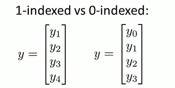
数和矩阵的乘法（标量乘法）

矩阵加法：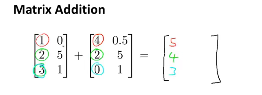

不同形式的矩阵由于维数不同所以无法相加

标量乘法：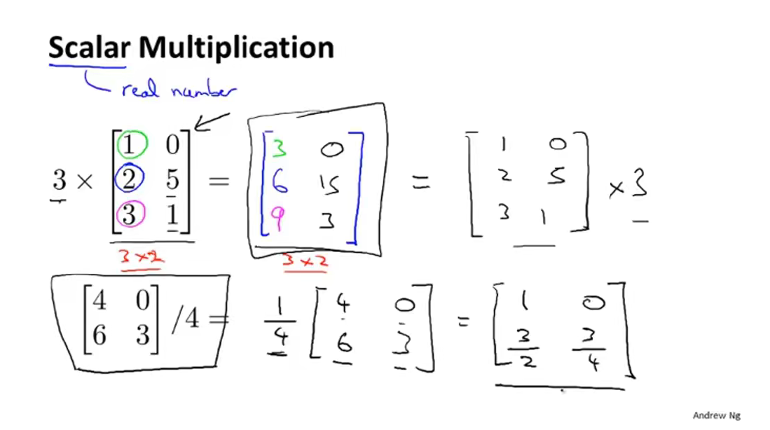

混合运算：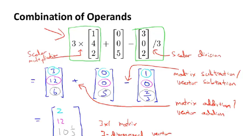

矩阵的乘法：

 

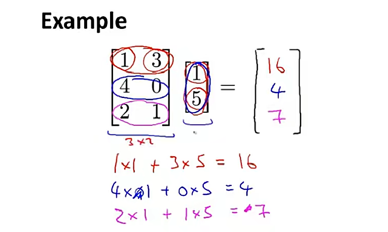
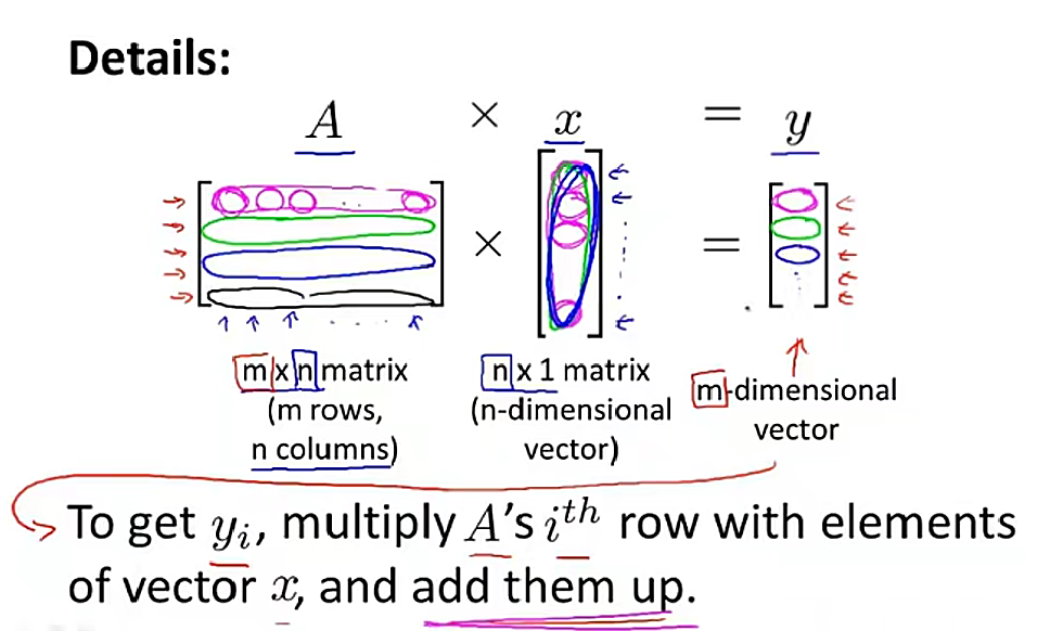
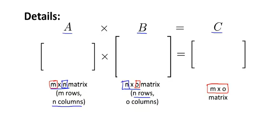
矩阵乘法特征：

不具备交换律

满足结合率

单位矩阵：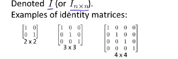

逆和转置

逆：类似于实数的倒数

只有方阵才有逆矩阵

不存在逆矩阵的矩阵被叫做奇异矩阵（退化矩阵）

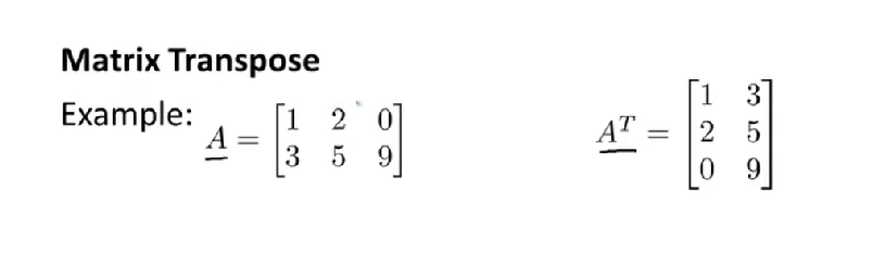
矩阵的转置运算：

第四章：

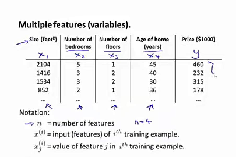
多变量线性回归

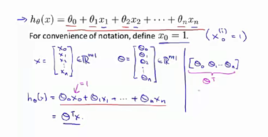
数学形式定义

 

参数求解：

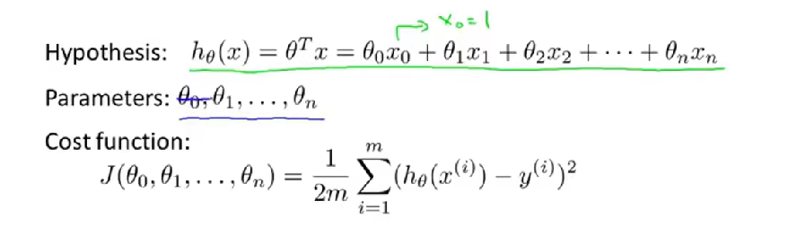
梯度下降算法的变化：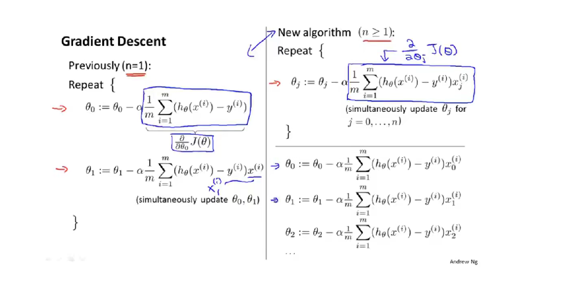

梯度下降运算中的实用技巧

1.特征缩放：

确保不同特征的取值在一个相似的范围中

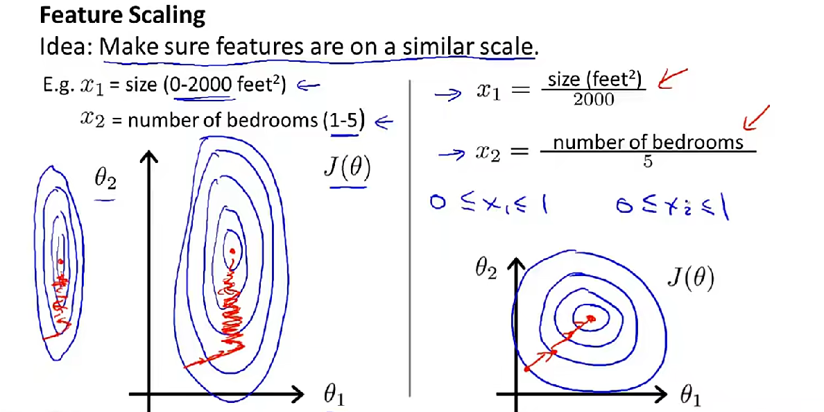
这样从数学的角度上就可以更快收敛。

进行特征缩放经常讲特征的取值放到-1到1之间。（这两个数并不是特别重要，接近就好）

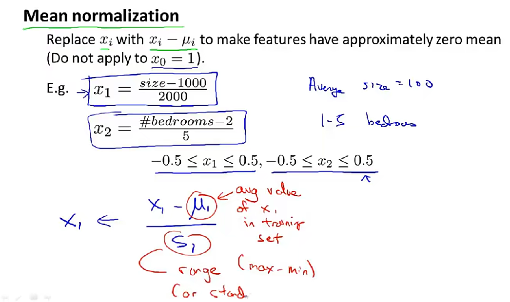
均值归一化：

2.学习率

学习率不要太大：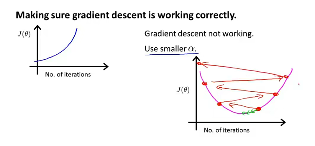

解决办法：选取一个较小的学习率的值

特征和多项式回归

多项式回归就类似于多变量回归，只不过x值之间存在关系

正规方程：
无需迭代，一次性求得参数的最优解

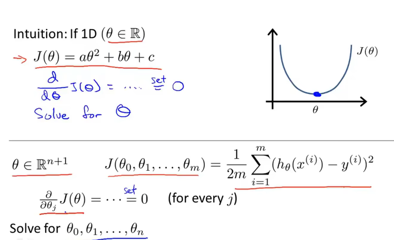
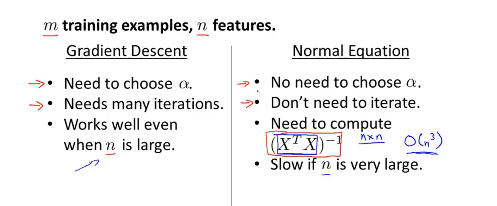
何时使用随机梯度下降算法，何时使用正规方程法

看特征的数量，如果特征的数量n很大，我们就选取梯度下降算法，如果n小的话，我们就可以采取正规方程的办法

正规方程以及其不可逆性

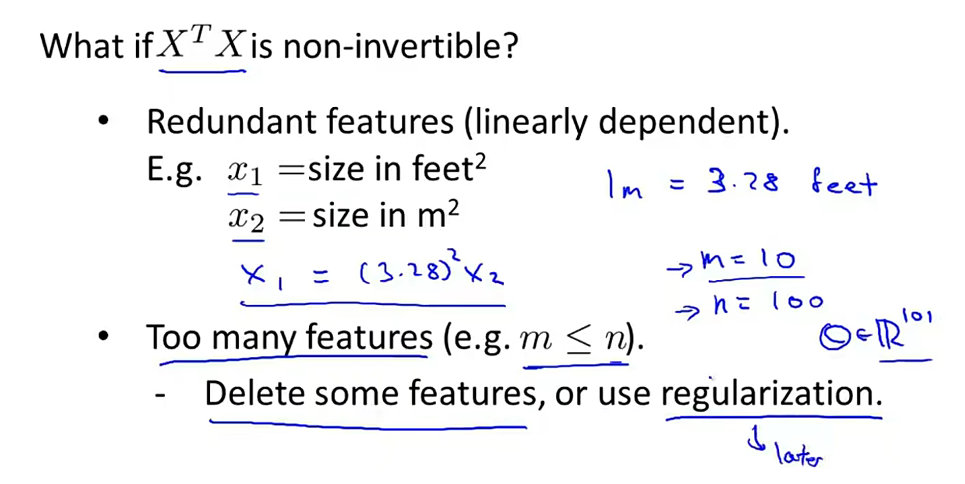
没有逆的情况：
1.特征之间存在线性关系，删除即可

2.特征太多了，数据集相对而言太少了，这时我们可以采用正则化的方式

---

代码实操：

import numpy as np
import matplotlib.pyplot as plt


# 从文件读取数据（假设数据格式：x1 x2 x3 y）
def load_data(filename):
    data = np.loadtxt(filename)
    X = data[:, :-1]  # 前三列作为特征
    y = data[:, -1]  # 最后一列作为目标值
    return X, y


# 计算误差均方函数 J(w,b)
def cost_function(X, y, w, b):
    m = X.shape[0]  # 训练集的数据样本数
    cost_sum = 0.0
    for i in range(m):
        f_wb = np.dot(w, X[i]) + b
        cost = (f_wb - y[i]) ** 2
        cost_sum += cost
    return cost_sum / (2 * m)


# 计算梯度值 dJ/dw, dJ/db
def compute_gradient(X, y, w, b):
    m, n = X.shape  # m: 样本数, n: 特征数
    d_w = np.zeros(n)  # 梯度向量，对应每个特征
    d_b = 0.0

    for i in range(m):
        # np.dot 是 NumPy 的“点积/矩阵乘法”函数
        error = np.dot(w, X[i]) + b - y[i]
        for j in range(n):
            d_w[j] += error * X[i, j]
        d_b += error

    dj_dw = d_w / m
    dj_db = d_b / m
    return dj_dw, dj_db


# 梯度下降算法
def gradient_descent(X, y, w, b, learning_rate=0.01, epochs=1000):
    J_history = []  # 记录每次迭代产生的误差值
    for epoch in range(epochs):
        dj_dw, dj_db = compute_gradient(X, y, w, b)
        # w 和 b 需同步更新
        w = w - learning_rate * dj_dw
        b = b - learning_rate * dj_db
        J_history.append(cost_function(X, y, w, b))  # 记录每次迭代产生的误差值

        # 每1000次迭代打印一次进度
        if epoch % 1000 == 0:
            print(f"Epoch {epoch}: Cost = {J_history[-1]:.6f}")

    return w, b, J_history


# 最小二乘法
def least_squares(X, y):
    # 添加一列全1，用于计算偏置项
    X_aug = np.column_stack((np.ones(X.shape[0]), X))
    # 矩阵拼接，增加一列
    # 计算最小二乘解：w' = (X'^T X')^{-1} X'^T y
    try:
        # 使用正规方程求解
        # 运算符 @ 在 NumPy 里就是矩阵乘法的语法
        w_prime = np.linalg.inv(X_aug.T @ X_aug) @ X_aug.T @ y
    except np.linalg.LinAlgError:
        # 如果矩阵不可逆，使用伪逆
        print("矩阵不可逆，使用伪逆求解")
        w_prime = np.linalg.pinv(X_aug) @ y

    # 提取偏置项和权重
    b = w_prime[0]
    w = w_prime[1:]

    return w, b


# 预测函数
def predict(X, w, b):
    return np.dot(X, w) + b


# 绘制每个特征与目标值的关系
def plot_features_vs_target(X, y, w, b, feature_names):
    n_features = X.shape[1]
    fig, axes = plt.subplots(1, n_features, figsize=(5 * n_features, 5))

    if n_features == 1:
        axes = [axes]

    for i in range(n_features):
        # 按当前特征排序
        sorted_indices = np.argsort(X[:, i])
        # 返回“排序后的下标”
        x_sorted = X[sorted_indices, i]
        # NumPy 的“花式索引”规则：
        # 第一个位置放 行号数组 (sorted_indices)
        # 第二个位置放 列号 (i)
        # 效果就是：
        # “先把整份数据按 sorted_indices 指定的行顺序重新排，再只拿第 i 列”。
        y_sorted = y[sorted_indices]

        # 绘制散点图
        axes[i].scatter(x_sorted, y_sorted, alpha=0.7, label='Actual')

        # 绘制预测线（固定其他特征为均值）
        x_line = np.linspace(x_sorted.min(), x_sorted.max(), 100)
        # 创建预测点，其他特征设为均值
        X_pred = np.tile(X.mean(axis=0), (100, 1))
        X_pred[:, i] = x_line
        y_pred = predict(X_pred, w, b)

        axes[i].plot(x_line, y_pred, 'r-', linewidth=2, label='Predicted')
        axes[i].set_xlabel(feature_names[i])
        axes[i].set_ylabel('Target')
        axes[i].set_title(f'{feature_names[i]} vs Target')
        axes[i].legend()
        axes[i].grid(True, alpha=0.3)

    plt.tight_layout()
    return fig


# 绘制实际值 vs 预测值
def plot_actual_vs_predicted(X, y, w, b, title_suffix=""):
    y_pred = predict(X, w, b)

    plt.figure(figsize=(8, 6))
    plt.scatter(y, y_pred, alpha=0.7)

    min_val = min(y.min(), y_pred.min())
    max_val = max(y.max(), y_pred.max())
    plt.plot([min_val, max_val], [min_val, max_val], 'r--', alpha=0.8)

    plt.xlabel('Actual Values')
    plt.ylabel('Predicted Values')
    plt.title(f'Actual vs Predicted Values {title_suffix}')
    plt.grid(True, alpha=0.3)

    # 计算R²分数
    r_squared = 1 - np.sum((y - y_pred) ** 2) / np.sum((y - np.mean(y)) ** 2)
    plt.text(0.05, 0.95, f'R² = {r_squared:.4f}', transform=plt.gca().transAxes,
             bbox=dict(boxstyle="round", facecolor='wheat', alpha=0.5))

    return plt.gcf()


# 绘制误差值的收敛曲线
def plot_convergence(J_history, epochs, title_suffix=""):
    plt.figure(figsize=(10, 6))
    plt.plot(range(epochs), J_history, 'b-', linewidth=1)
    plt.xlabel('Epochs', size=15)
    plt.ylabel('Cost', size=15)
    plt.title(f'Cost Function Convergence {title_suffix}', size=20)
    plt.grid(True, alpha=0.3)
    plt.yscale('log')  # 使用对数坐标更好地显示收敛
    return plt.gcf()

# 比较两种方法的结果
def compare_methods(X, y, w_gd, b_gd, w_ls, b_ls):
    print("\n=== 方法比较 ===")
    print("梯度下降法结果:")
    for i in range(len(w_gd)):
        print(f"  w{i + 1} = {w_gd[i]:.6f}")
    print(f"  b = {b_gd:.6f}")

    print("\n最小二乘法结果:")
    for i in range(len(w_ls)):
        print(f"  w{i + 1} = {w_ls[i]:.6f}")
    print(f"  b = {b_ls:.6f}")

    # 计算两种方法的成本
    cost_gd = cost_function(X, y, w_gd, b_gd)
    cost_ls = cost_function(X, y, w_ls, b_ls)

    print(f"\n成本比较:")
    print(f"  梯度下降法: {cost_gd:.6f}")
    print(f"  最小二乘法: {cost_ls:.6f}")
    print(f"  差异: {abs(cost_gd - cost_ls):.6f}")

    # 计算R²分数
    y_pred_gd = predict(X, w_gd, b_gd)
    y_pred_ls = predict(X, w_ls, b_ls)
    # 1-RSS（残差平方和)/TSS（总平方和）
    r2_gd = 1 - np.sum((y - y_pred_gd) ** 2) / np.sum((y - np.mean(y)) ** 2)
    r2_ls = 1 - np.sum((y - y_pred_ls) ** 2) / np.sum((y - np.mean(y)) ** 2)

    print(f"\nR²分数比较:")
    print(f"  梯度下降法: {r2_gd:.6f}")
    print(f"  最小二乘法: {r2_ls:.6f}")
    print(f"  差异: {abs(r2_gd - r2_ls):.6f}")


# 从这里开始执行
if __name__ == '__main__':
    # 从文件读取数据
    X_train, y_train = load_data('multiple_variable.txt')
    # f 或 F 前缀告诉 Python，这是一个格式化字符串，大括号 {} 内的表达式会被求值并替换为对应的值。
    print(f"成功加载数据: {X_train.shape[0]} 个样本, {X_train.shape[1]} 个特征")
    # shape是Numpy数组的一个非常重要的属性，返回一个元组，0是行，1是列
    print(f"X数据范围: ")
    for i in range(X_train.shape[1]):
        print(f"  特征 {i + 1}: {X_train[:, i].min():.2f} - {X_train[:, i].max():.2f}")
    print(f"y数据范围: {y_train.min():.2f} - {y_train.max():.2f}")
    # :.2f 告诉 Python “把刚才那个值格式化成保留 2 位小数的浮点数”。

    # 初始化参数
    n_features = X_train.shape[1]
    feature_names = [f'X{i + 1}' for i in range(n_features)]

    # 方法1: 梯度下降法
    print("\n=== 使用梯度下降法 ===")
    w_gd = np.zeros(n_features)  # 权重向量
    b_gd = 0.0  # 偏置
    epochs = 10000  # 迭代次数
    learning_rate = 0.02  # 学习率（可能需要调整）

    w_gd, b_gd, J_history = gradient_descent(X_train, y_train, w_gd, b_gd, learning_rate, epochs)

    # 方法2: 最小二乘法
    print("\n=== 使用最小二乘法 ===")
    w_ls, b_ls = least_squares(X_train, y_train)

    # 比较两种方法
    compare_methods(X_train, y_train, w_gd, b_gd, w_ls, b_ls)

    # 可视化梯度下降法的结果
    plot_features_vs_target(X_train, y_train, w_gd, b_gd, feature_names)
    plt.show()

    plot_actual_vs_predicted(X_train, y_train, w_gd, b_gd, "(Gradient Descent)")
    plt.show()

    plot_convergence(J_history, epochs, "(Gradient Descent)")
    plt.show()

    # 可视化最小二乘法的结果
    plot_features_vs_target(X_train, y_train, w_ls, b_ls, feature_names)
    plt.show()

    plot_actual_vs_predicted(X_train, y_train, w_ls, b_ls, "(Least Squares)")
    plt.show()