使用机器学习方法对高光谱进行分类

高光谱图像（Hyperspectral Image, HSI）具有丰富的光谱信息，能够对地物进行精细分类。然而，其高维特性也带来了"维度灾难"等挑战。支持向量机（Support Vector Machine, SVM）作为一种经典的机器学习方法，在高光谱分类任务中表现出色。

本文通过Python实现SVM对高光谱图像的分类过程，主要步骤包括：数据预处理、特征提取、模型训练与评估。代码基于scikit-learn库实现，完整展示了从数据加载到分类结果可视化的全流程。

## 数据准备与可视化
# 导入必要的库
import numpy as np
import pandas as pd
import seaborn as sns
import matplotlib.pyplot as plt
from scipy.io import loadmat  # 用于加载.mat格式的MATLAB数据文件

# 加载Indian Pines高光谱数据集
# 该数据集是美国印第安纳州西北部农田地区的高光谱图像
# 包含145x145像素，224个光谱波段(0.4-2.5微米)
X = loadmat('./dataset/Indian_pines_corrected.mat')['indian_pines_corrected']  # 原始光谱数据
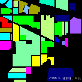
y = loadmat('./dataset/Indian_pines_gt.mat')['indian_pines_gt']  # 地面真实标签数据

# 定义类别标签与其对应的名称
# 该数据集包含16种不同的地表覆盖类型
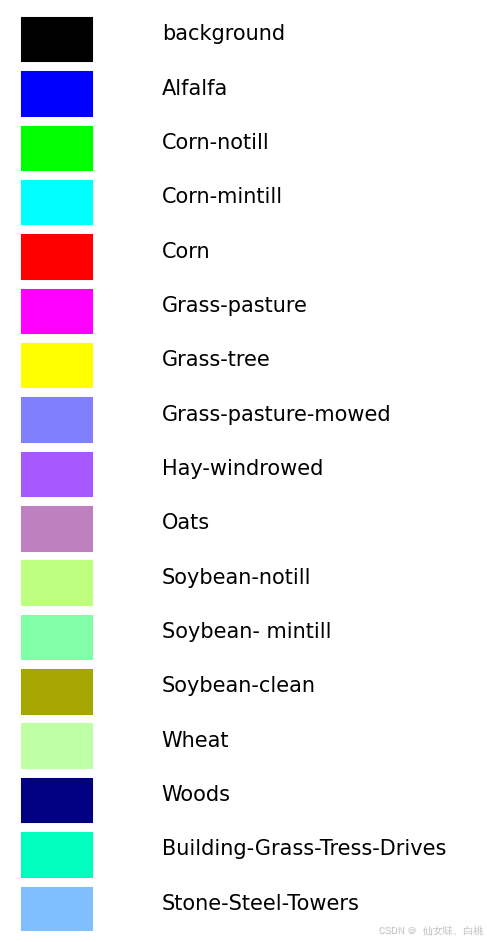
class_labels = {
    '1':'Alfalfa',  # 苜蓿
    '2':'Corn-notill',  # 免耕玉米
    '3':'Corn-mintill',  # 少耕玉米
    '4':'Corn',  # 传统耕作玉米
    '5':'Grass-pasture',  # 牧草
    '6':'Grass-trees',  # 草地树木
    '7':'Grass-pasture-mowed',  # 割草牧草
    '8':'Hay-windrowed',  # 干草
    '9':'Oats',  # 燕麦
    '10':'Soybean-notill',  # 免耕大豆
    '11':'Soybean-mintill',  # 少耕大豆
    '12':'Soybean-clean',  # 传统耕作大豆
    '13':'Wheat',  # 小麦
    '14':'Woods',  # 林地
    '15':'Buildings-Grass-Trees-Drives',  # 建筑-草地-树木-道路
    '16':'Stone-Steel-Towers',  # 石钢塔
}

# 将类别名称存储在列表中便于后续可视化
names = [
    'Alfalfa', 'Corn-notill', 'Corn-mintill', 'Corn', 
    'Grass-pasture', 'Grass-trees', 'Grass-pasture-mowed', 
    'Hay-windrowed', 'Oats', 'Soybean-notill', 'Soybean-mintill',
    'Soybean-clean', 'Wheat', 'Woods', 
    'Buildings Grass Trees Drives', 'Stone Steel Towers'
]

## 使用SVM进行分类
from sklearn.preprocessing import StandardScaler  # 用于数据标准化
from sklearn.model_selection import train_test_split  # 数据集划分工具
from sklearn.svm import SVC  # SVM分类器
from sklearn.metrics import accuracy_score, classification_report, confusion_matrix  # 评估指标
import pandas as pd  # 数据处理
import numpy as np  # 数值计算
import matplotlib.pyplot as plt  # 可视化
import seaborn as sns  # 高级可视化

# 光谱数据预处理步骤
# 将3D光谱数据(X)展平为2D格式(样本数×波段数)
# 同时将标签数据(y)保存为CSV文件
# 具体操作：
# 1. 首先保存纯净的标签数据
pd.DataFrame(y).to_csv("df_indian_pines_gt.csv", index=False)  

# 2. 将光谱数据重塑为(样本数×波段数)的2D格式
q = X.reshape(-1, X.shape[2])  

# 3. 创建包含所有波段的数据框
df = pd.DataFrame(q)  

# 4. 将标签数据展平并合并到特征数据中
df = pd.concat([df, pd.DataFrame(y.ravel())], axis=1)  

# 5. 设置列名(波段1到波段N + 类别列)
df.columns = [f'band{i}' for i in range(1, 1+X.shape[2])] + ['class']  

# 6. 保存完整数据集
df.to_csv('indian_pines_all.csv', index=False)  

def svm_matrix_plot(X, y, names):
    """
    使用SVM对高光谱数据进行分类，可视化混淆矩阵，并输出分类指标
    ----
    参数:
    X: 特征数据，形状为(样本数, 特征数)的numpy数组
    y: 标签数据，形状为(样本数,)的numpy数组
    names: 类别名称列表
    
    返回:
    svm: 训练好的SVM模型
    y_test: 测试集真实标签
    ypred: 测试集预测结果
    
    处理流程:
    1. 数据划分(80%训练，20%测试)
    2. SVM模型训练(使用RBF核)
    3. 模型预测
    4. 混淆矩阵可视化
    """
    # 1. 数据划分 - 保持类别分布(stratify)
    X_train, X_test, y_train, y_test = train_test_split(
        X, y, 
        test_size=0.20, 
        random_state=11, 
        stratify=y
    )
    
    # 2. 初始化SVM分类器
    # 使用RBF核，正则化参数C=100
    # 设置大缓存(10MB)提高训练速度
    svm = SVC(
        C=100, 
        kernel='rbf', 
        cache_size=10*1024
    )
    
    # 3. 模型训练
    svm.fit(X_train, y_train)
    
    # 4. 模型预测
    ypred = svm.predict(X_test)
    
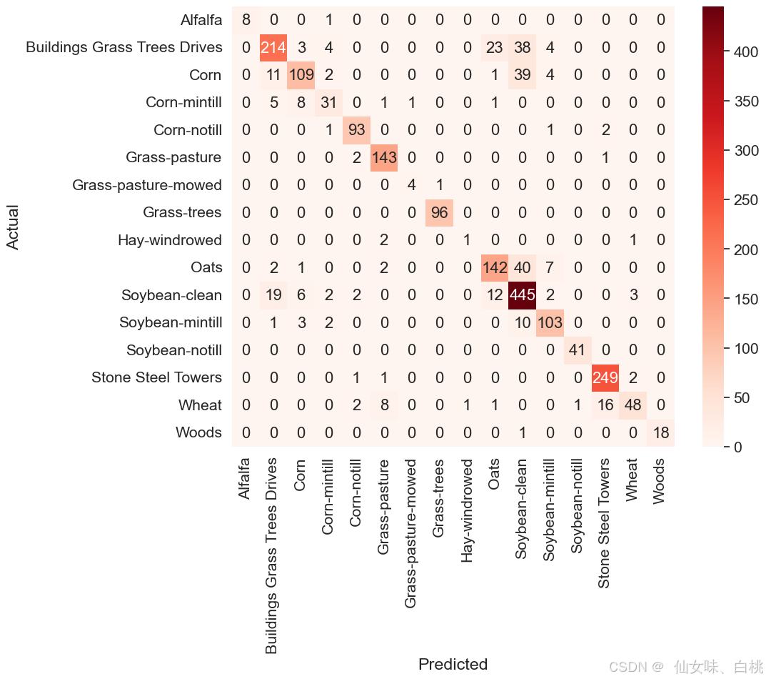
    # 5. 混淆矩阵计算
    conf_matrix = confusion_matrix(y_test, ypred)
    
    # 6. 创建美观的DataFrame格式混淆矩阵
    df_cm = pd.DataFrame(
        conf_matrix, 
        columns=np.unique(names), 
        index=np.unique(names)
    )
    df_cm.index.name = 'Actual'
    df_cm.columns.name = 'Predicted'
    
    # 7. 可视化混淆矩阵
    plt.figure(figsize=(10, 8))
    sns.set(font_scale=1.4)  # 设置标签大小
    sns.heatmap(
        df_cm, 
        cmap="Reds", 
        annot=True,  # 显示数值
        annot_kws={"size": 16},  # 数值大小
        fmt='d'  # 整数格式
    )
    
    return svm, y_test, ypred

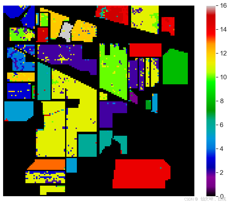
def plot_classify(svm, q, save_name='IP_cmap'):
    """
    绘制分类结果可视化图
    ----
    Parameters:
    svm : 已训练好的SVM分类器模型
        用于对新数据进行预测的分类器对象
    q : pandas.DataFrame
        包含待分类数据的数据框，最后一列为类别标签
    save_name : str, optional
        保存图像的文件名前缀（默认值为'IP_cmap'）
        
    Returns:
    None
        直接显示并保存分类结果图像
    """
    # 初始化结果列表
    l = []
    
    # 遍历数据集中的每个样本
    for i in range(q.shape[0]):
        # 背景类（标签为0）直接标记为0
        if q.iloc[i, -1] == 0:
            l.append(0)
        else:
            # 非背景类使用SVM进行预测
            sample = q.iloc[i, :-1].values.reshape(1, -1)  # 转换为2D数组
            prediction = svm.predict(sample)[0]  # 获取预测结果
            l.append(prediction)
    
    # 将结果列表转换为145x145的numpy数组
    clmap = np.array(l).reshape(145, 145).astype('float')
    
    # 创建图像
    plt.figure(figsize=(10, 8))
    # 使用nipy_spectral色彩映射显示分类结果
    plt.imshow(clmap, cmap='nipy_spectral')
    # 添加颜色条
    plt.colorbar()
    # 不显示坐标轴
    plt.axis('off')
    # 保存图像到results目录下
    plt.savefig(f'./results/{save_name}.png', dpi=300, bbox_inches='tight')
    # 显示图像
    plt.show()

# 重新读取Indian Pines数据集
# 该数据集包含145×145像素的高光谱图像，共200个波段
# 最后一列为类别标签（0表示背景，1-16表示不同地物类别）
df = pd.read_csv('indian_pines_all.csv')

# 查看数据集的基本信息
print(f"数据集形状: {df.shape}")
print(f"波段数量: {df.shape[1]-1}")  # 减去标签列
print("类别分布:")
print(df['class'].value_counts())

# 显示数据集前5行
# 可以查看各波段数值范围和标签信息
df.head()

# 数据预处理：去除背景（0类）样本
# 背景样本不参与分类模型训练和评估
x = df[df['class'] != 0]  # 筛选非背景样本
X = x.iloc[:, :-1].values  # 提取特征数据（200个波段）
y = x.iloc[:, -1].values   # 提取标签数据

# 输出处理后数据信息
print(f"有效样本数: {X.shape[0]}")
print(f"特征维度: {X.shape[1]}")
print(f"类别数: {len(np.unique(y))}")

# 调用SVM分类方法进行模型训练和预测
# 该函数返回训练好的SVM模型、测试集真实标签和预测标签
svm, y_test, ypred = svm_matrix_plot(X, y)

# 可选：打印分类性能指标
from sklearn.metrics import classification_report
print(classification_report(y_test, ypred))

print(classification_report(y_test, ypred, target_names = names)) # 打印分类结果

                              precision    recall  f1-score   support

                     Alfalfa       1.00      0.89      0.94         9
                 Corn-notill       0.85      0.75      0.80       286
                Corn-mintill       0.84      0.66      0.74       166
                        Corn       0.72      0.66      0.69        47
               Grass-pasture       0.93      0.96      0.94        97
                 Grass-trees       0.91      0.98      0.94       146
         Grass-pasture-mowed       0.80      0.80      0.80         5
               Hay-windrowed       0.99      1.00      0.99        96
                        Oats       0.50      0.25      0.33         4
              Soybean-notill       0.79      0.73      0.76       194
             Soybean-mintill       0.78      0.91      0.84       491
               Soybean-clean       0.85      0.87      0.86       119
                       Wheat       0.98      1.00      0.99        41
                       Woods       0.93      0.98      0.96       253
Buildings Grass Trees Drives       0.89      0.62      0.73        77
          Stone Steel Towers       1.00      0.95      0.97        19

                    accuracy                           0.85      2050
                   macro avg       0.86      0.81      0.83      2050
                weighted avg       0.85      0.85      0.85      2050

# 可视化分类结果
plot_classify(svm, df, save_name = 'IP_SVM_Orig')

## 使用PCA降维，然后分类

from sklearn.decomposition import PCA

pca_components = 50
pca = PCA(n_components = pca_components)
data = df.iloc[:, :-1].values
dt = pca.fit_transform(data)

# 将降维之后的光谱和类别进行拼接创建一个新的数据
q = pd.concat([pd.DataFrame(data = dt), pd.DataFrame(df.iloc[:, -1])], axis = 1)
q.columns = [f'PC-{i}' for i in range(1, pca_components+1)]+['class']

q.head()

	PC-1	PC-2	PC-3	PC-4	PC-5	PC-6	PC-7	PC-8	PC-9	PC-10	...	PC-42	PC-43	PC-44	PC-45	PC-46	PC-47	PC-48	PC-49	PC-50	class
0	5014.905985	-1456.863260	72.697049	71.204926	-435.686985	-68.840318	-134.809864	304.372455	256.432994	66.630999	...	7.219730	-67.989578	98.721564	25.095257	46.913222	4.976732	23.604549	-29.224580	-69.679783	3
1	5601.383743	2023.450087	350.134661	-528.465053	148.088296	-288.359031	-202.956863	-240.848020	-474.857836	-93.493771	...	-8.325960	-14.802372	48.198445	-56.200235	9.298071	-1.941736	-14.542037	-24.024475	-67.698322	3
2	5796.135442	3090.394852	490.539929	-760.214346	259.933303	-131.611181	-172.927304	-205.911237	572.491978	191.622014	...	6.052947	11.751196	-13.271799	-137.887551	27.103948	36.394854	36.495065	-20.268499	-58.394823	3
3	5586.204575	2369.376085	356.274719	-502.687155	146.554951	-306.679326	-251.071095	-234.966433	-314.023248	-54.962246	...	28.289417	-29.190102	74.136672	-6.903011	44.521142	14.325024	-6.531956	20.396631	-48.922193	3
4	5020.990792	-339.603390	-23.007525	-92.556769	-368.495443	-438.266709	-502.715429	345.536587	-188.352757	67.506061	...	46.756325	-101.560795	139.485647	99.365248	68.453213	19.267719	29.546286	70.415027	-37.565652	3

5 rows × 51 columns

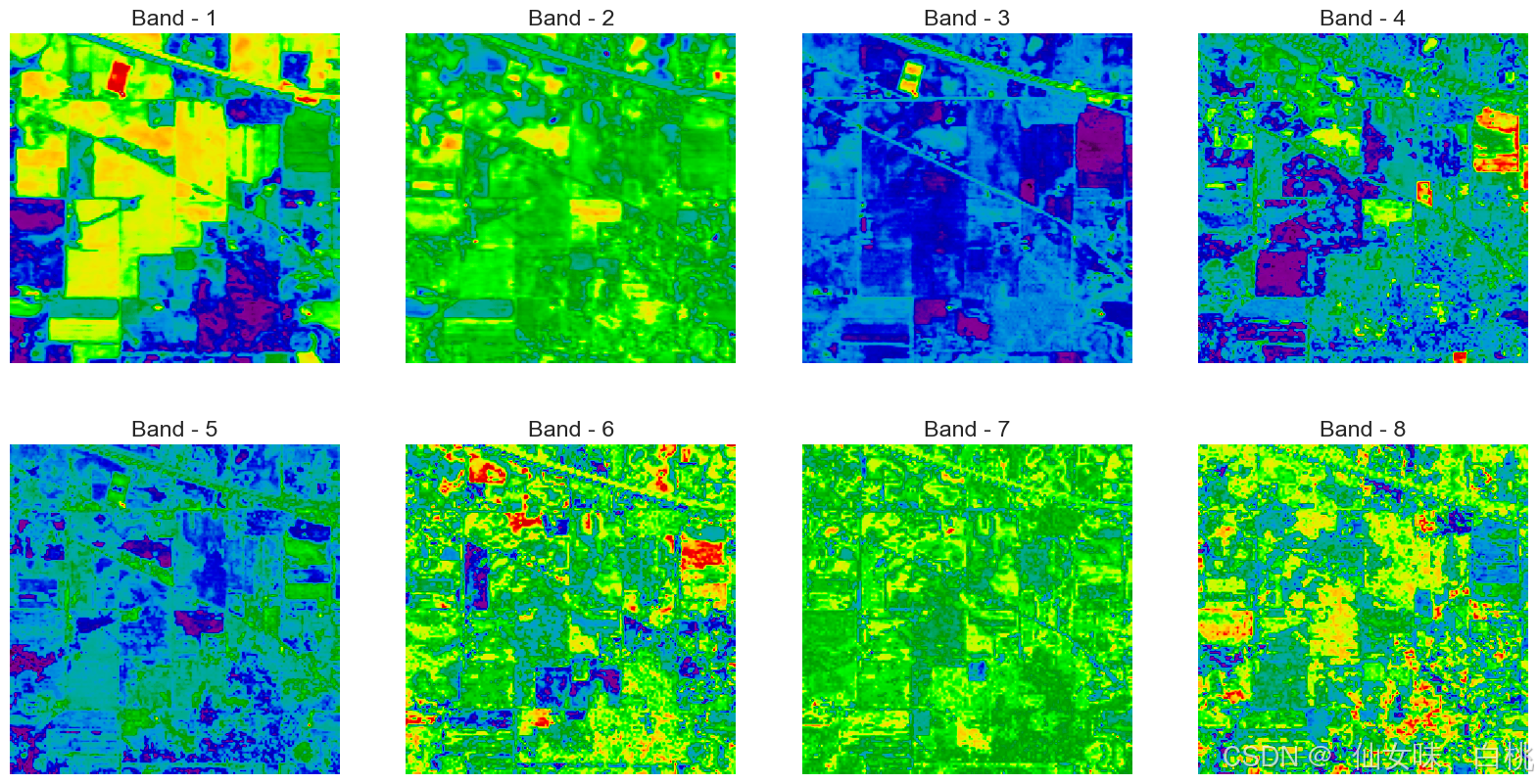
# 将降维之后的光谱数据进行可视化
def plot_pca(q):
    fig = plt.figure(figsize = (20, 10))
    for i in range(1, 1+8):
        fig.add_subplot(2,4, i)
        plt.imshow(q.loc[:, f'PC-{i}'].values.reshape(145, 145), cmap='nipy_spectral')
        plt.axis('off')
        plt.title(f'Band - {i}')

plot_pca(q)

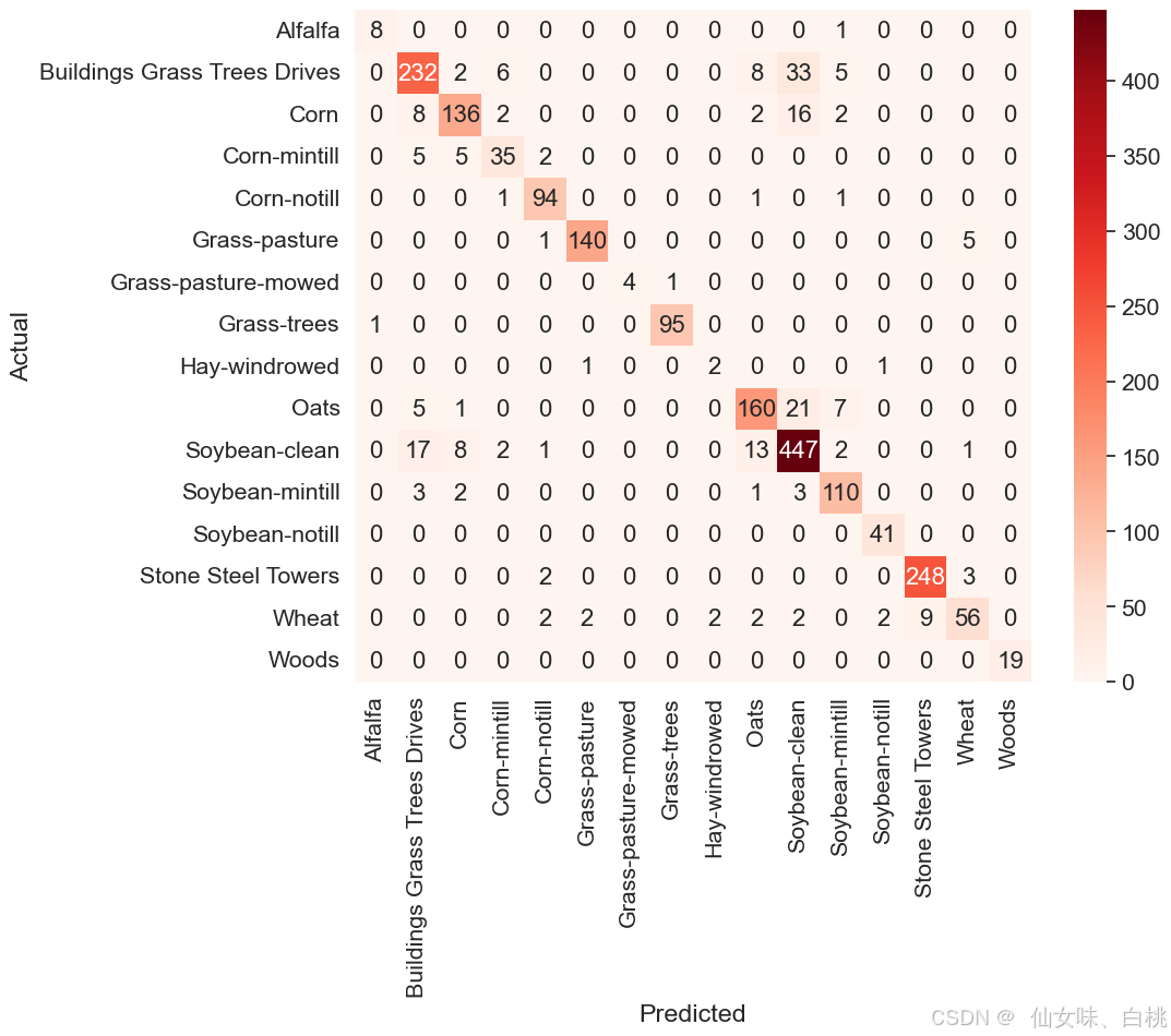
# 使用降维之后的数据重新进行分类
# 去除掉背景（0类）
x = q[q['class'] != 0]
X = x.iloc[:, :-1].values
y = x.loc[:, 'class'].values

svm, y_test, ypred = svm_matrix_plot(X, y)

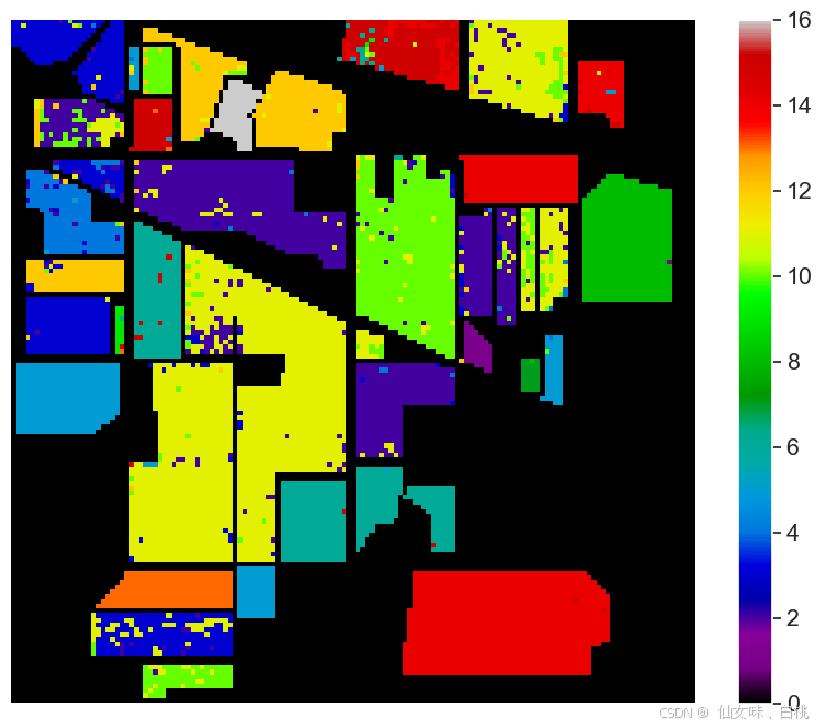
# 绘制降维之后的数据分类结果
plot_classify(svm, q, save_name = 'IP_SVM_PCA')