[机器学习-从入门到入土] 神经网络
[机器学习-从入门到入土] 神经网络
个人导航
知乎:https://www.zhihu.com/people/byzh_rc
CSDN:https://blog.csdn.net/qq_54636039
注:本文仅对所述内容做了框架性引导,具体细节可查询其余相关资料or源码
目录
neural-networks.ipynb
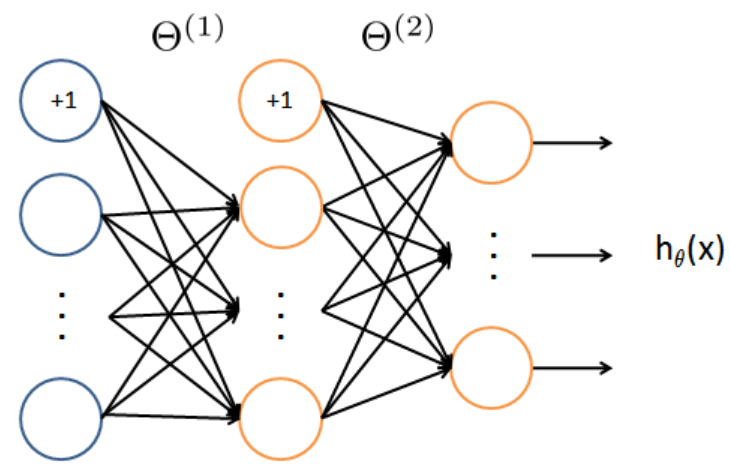
神经网络是一个三层的结构(一个输入层,一个隐藏层,一个输出层)
输入层单元数为400(考虑偏置为401)
隐藏层单元数为25(考虑偏置为26)
输出层单元数为10(K=10个类别)
输入层->隐藏层:
Θ
(
1
)
:
s
h
a
p
e
=
(
h
i
d
d
e
n
_
s
i
z
e
,
1
+
i
n
p
u
t
_
s
i
z
e
)
\Theta^{(1)}: shape=(hidden\_size, 1+input\_size)
Θ(1):shape=(hidden_size,1+input_size)
隐藏层->输出层:
Θ
(
2
)
:
s
h
a
p
e
=
(
n
u
m
_
l
a
b
e
l
s
,
1
+
h
i
d
d
e
n
_
s
i
z
e
)
\Theta^{(2)}: shape=(num\_labels, 1+hidden\_size)
Θ(2):shape=(num_labels,1+hidden_size)
y y y使用了one-hot的表达方式: ( y k y_k yk代表第k类, 是为1, 不是为0)
y_one_hot = np.zeros((m, num_labels))
y_one_hot[np.arange(m), y.flatten() - 1] = 1
# y: (m, 1) 数值从1到10
# -> y_one_hot: (m, num_labels)
1.sigmoid
Sigmoid 函数定义为:
sigmoid
(
z
)
=
g
(
z
)
=
1
1
+
exp
(
−
z
)
\text{sigmoid}(z) = g(z) = \frac{1}{1+\exp(-z)}
sigmoid(z)=g(z)=1+exp(−z)1
Sigmoid 函数的梯度可以按照下式进行计算:
g
′
(
z
)
=
d
d
z
g
(
z
)
=
g
(
z
)
(
1
−
g
(
z
)
)
g^{\prime}(z) = \frac{d}{dz} g(z) = g(z)(1-g(z))
g′(z)=dzdg(z)=g(z)(1−g(z))
2.网络参数的随机初始化
一个非常有效的随机初始化策略为,在范围 [ − ϵ i n i t , ϵ i n i t ] [ -\epsilon_{init}, \epsilon_{init} ] [−ϵinit,ϵinit] 内按照均匀分布随机选择参数 Θ ( l ) \Theta^{(l)} Θ(l) 的初始值
对于一般的神经网络,如果第
l
l
l 层的输入单元数为
L
i
n
L_{in}
Lin ,输出单元数为
L
o
u
t
L_{out}
Lout
则
ϵ
i
n
i
t
=
6
/
L
i
n
+
L
o
u
t
\epsilon_{init} = {\sqrt{6}}/{\sqrt{L_{in} + L_{out}}}
ϵinit=6/Lin+Lout 可以做为有效的指导策略
ϵ
i
n
i
t
=
6
L
i
n
+
L
o
u
t
\epsilon_{init} = \frac{\sqrt{6}}{\sqrt{L_{in} + L_{out}}}
ϵinit=Lin+Lout6
这里设置 ϵ i n i t = 0.12 \epsilon_{init}=0.12 ϵinit=0.12
3.代价函数Cost Function
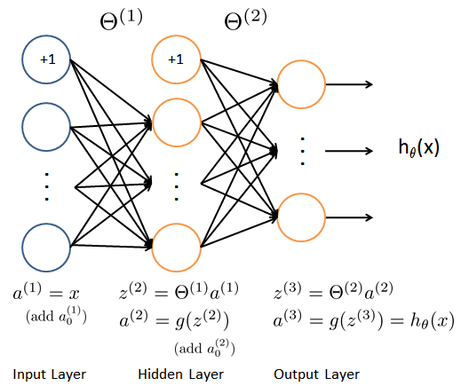
神经网络的代价函数(不包括正则化项)的定义为:
J
(
θ
)
=
1
m
∑
i
=
1
m
∑
k
=
1
K
−
y
k
(
i
)
log
(
(
h
θ
(
x
(
i
)
)
)
k
)
J(\theta) = \frac{1}{m} \sum_{i=1}^{m} \sum_{k=1}^{K} -y_k^{(i)} \log\left((h_{\theta}(x^{(i)}))_k\right)
J(θ)=m1i=1∑mk=1∑K−yk(i)log((hθ(x(i)))k)
a1 = np.c_[np.ones((m, 1)), X]
z2 = a1 @ Theta1.transpose(1, 0)
a2 = np.c_[np.ones((m, 1)), sigmoid(z2)]
z3 = a2 @ Theta2.transpose(1, 0)
a3 = sigmoid(z3)
h = a3
J += lmb / (2*m) * (np.sum(Theta1[:, 1:]**2) + np.sum(Theta2[:, 1:]**2))
# Theta1: (hidden, 1+input_size) Theta2: (num_labels, 1+hidden)
# X: (m, input_size) a1: (m, 1+input_size)
# z2: (m, hidden) a2: (m, 1+hidden)
# z3: (m, num_labels) a3/h: (m, num_labels)
# -> J: 数
神经网络包括正则化项的代价函数为:
J
(
θ
)
=
1
m
∑
i
=
1
m
∑
k
=
1
K
−
y
k
(
i
)
log
(
(
h
θ
(
x
(
i
)
)
)
k
)
+
λ
2
m
[
∑
j
=
1
25
∑
k
=
1
400
(
Θ
j
,
k
(
1
)
)
2
+
∑
j
=
1
10
∑
k
=
1
25
(
Θ
j
,
k
(
2
)
)
2
]
J(\theta) = \frac{1}{m}\sum_{i=1}^{m} \sum_{k=1}^{K} -y_k^{(i)} \log\left((h_{\theta}(x^{(i)}))_k\right) + \frac{\lambda}{2m} \left[\sum_{j=1}^{25} \sum_{k=1}^{400} (\Theta_{j,k}^{(1)})^2 +\sum_{j=1}^{10} \sum_{k=1}^{25} (\Theta_{j,k}^{(2)})^2 \right]
J(θ)=m1i=1∑mk=1∑K−yk(i)log((hθ(x(i)))k)+2mλ[j=1∑25k=1∑400(Θj,k(1))2+j=1∑10k=1∑25(Θj,k(2))2]
偏置项的参数不能包括在正则化项中
对于矩阵Theta1与Theta2而言,偏置项对应于矩阵的第一列
J += lmb / (2*m) * (np.sum(Theta1[:, 1:]**2) + np.sum(Theta2[:, 1:]**2))
# -> J: 数
4.(误差)反向传播Error Backpropagation
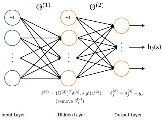
对于一个训练样本 ( x ( t ) , y ( t ) ) (x^{(t)}, y^{(t)}) (x(t),y(t)) ,我们首先使用前向传播计算网络中所有神经元的激活值
对于第
l
l
l 层的第
j
j
j 个节点,计算出一个**“误差项”
δ
j
(
l
)
\delta_{j}^{(l)}
δj(l)** 用于衡量该节点对于输出的误差的“贡献”
隐藏层:
δ
(
2
)
:
s
h
a
p
e
=
(
m
,
h
i
d
d
e
n
_
s
i
z
e
)
\delta^{(2)}: shape=(m,hidden\_size)
δ(2):shape=(m,hidden_size)
输出层:
δ
(
3
)
:
s
h
a
p
e
=
(
m
,
n
u
m
_
l
a
b
e
l
s
)
\delta^{(3)}: shape=(m, num\_labels)
δ(3):shape=(m,num_labels)
累加后 -> 代价函数的总梯度是
Δ
(
l
)
\Delta^{(l)}
Δ(l)
输入层->隐藏层:
Δ
(
1
)
:
s
h
a
p
e
=
(
h
i
d
d
e
n
_
s
i
z
e
,
1
+
i
n
p
u
t
_
s
i
z
e
)
\Delta^{(1)}: shape=(hidden\_size, 1+input\_size)
Δ(1):shape=(hidden_size,1+input_size)
隐藏层->输出层:
Δ
(
2
)
:
s
h
a
p
e
=
(
n
u
m
_
l
a
b
e
l
s
,
1
+
h
i
d
d
e
n
_
s
i
z
e
)
\Delta^{(2)}: shape=(num\_labels, 1+hidden\_size)
Δ(2):shape=(num_labels,1+hidden_size)
对于输出节点: (直接计算网络的激活值与真实目标值之间的误差)
δ
k
(
3
)
=
a
k
(
3
)
−
y
k
k
=
0
,
.
.
.
,
n
u
m
_
l
a
b
e
l
s
−
1
δ
(
3
)
=
a
(
3
)
−
y
\delta_{k}^{(3)} = a_{k}^{(3)} - y_k \quad k=0, ..., num\_labels-1 \\ \delta^{(3)} = a^{(3)} - y
δk(3)=ak(3)−ykk=0,...,num_labels−1δ(3)=a(3)−y
根据sigmoid求导:
∂ a k ( 3 ) ∂ z k ( 3 ) = a k ( 3 ) ( 1 − a k ( 3 ) ) \frac{\partial a_k^{(3)}}{\partial z_k^{(3)}} = a_k^{(3)} (1 - a_k^{(3)}) ∂zk(3)∂ak(3)=ak(3)(1−ak(3))
根据CrossEntropy求导:
∂ J ∂ a k ( 3 ) = − 1 m ( y k a k ( 3 ) − 1 − y k 1 − a k ( 3 ) ) \frac{\partial J}{\partial a_k^{(3)}} = -\frac{1}{m} \left( \frac{y_k}{a_k^{(3)}} - \frac{1 - y_k}{1 - a_k^{(3)}} \right) ∂ak(3)∂J=−m1(ak(3)yk−1−ak(3)1−yk)
故:
δ k ( 3 ) = ∂ J ∂ z k ( 3 ) = ∂ J ∂ a k ( 3 ) ⋅ ∂ a k ( 3 ) ∂ z k ( 3 ) = a k ( 3 ) − y k \delta_k^{(3)} = \frac{\partial J}{\partial z_k^{(3)}} = \frac{\partial J}{\partial a_k^{(3)}} \cdot \frac{\partial a_k^{(3)}}{\partial z_k^{(3)}} = a_k^{(3)} - y_k δk(3)=∂zk(3)∂J=∂ak(3)∂J⋅∂zk(3)∂ak(3)=ak(3)−yk
delta3 = a3 - y_one_hot
# y_one_hot: (m, num_labels)
# a3: (m, num_labels)
# -> delta3: (m, num_labels)
对于隐层节点:
δ k ( 2 ) = g ′ ( z k ( 2 ) ) ∑ j = 0 n u m _ l a b e l s − 1 Θ j k ( 2 ) δ j ( 3 ) , k = 0 , … , hidden − 1 δ ( 2 ) = ( Θ ( 2 ) ) T δ ( 3 ) . ∗ g ′ ( z ( 2 ) ) \delta_k^{(2)} = g'\big(z_k^{(2)}\big) \sum_{j=0}^{num\_labels-1} \Theta_{jk}^{(2)} \, \delta_j^{(3)}, \quad k = 0, \dots, \text{hidden}-1 \\ \delta^{(2)} = \left( \Theta^{(2)} \right)^T \delta^{(3)} .* g^{\prime} (z^{(2)}) δk(2)=g′(zk(2))j=0∑num_labels−1Θjk(2)δj(3),k=0,…,hidden−1δ(2)=(Θ(2))Tδ(3).∗g′(z(2))
.*在numpy中是逐元素相乘
定义:
δ ( 3 ) = △ ∂ J ∂ z ( 2 ) = ∂ J ∂ a ( 2 ) ⋅ ∂ a ( 2 ) ∂ z ( 2 ) \delta^{(3)} \stackrel{\triangle}{=} \frac{\partial J}{\partial z^{(2)}}=\frac{\partial J}{\partial a^{(2)}}\cdot\frac{\partial a^{(2)}}{\partial z^{(2)}} δ(3)=△∂z(2)∂J=∂a(2)∂J⋅∂z(2)∂a(2)
由 z ( 3 ) = Θ ( 2 ) a ( 2 ) z^{(3)} = \Theta^{(2)} a^{(2)} z(3)=Θ(2)a(2)可得:
∂ J ∂ a ( 2 ) = ( Θ ( 2 ) ) T ∂ J ∂ z ( 3 ) = ( Θ ( 2 ) ) T δ ( 3 ) \frac{\partial J}{\partial a^{(2)}} = \left( \Theta^{(2)} \right)^{T} \frac{\partial J}{\partial z^{(3)}} =\left( \Theta^{(2)} \right)^{T}\delta^{(3)} ∂a(2)∂J=(Θ(2))T∂z(3)∂J=(Θ(2))Tδ(3)
由sigmoid求导可得:
∂ a ( 2 ) ∂ z ( 2 ) = g ′ ( z ( 2 ) ) \frac{\partial a^{(2)}}{\partial z^{(2)}} = g^{\prime} (z^{(2)}) ∂z(2)∂a(2)=g′(z(2))
part1 = (delta3 @ Theta2)[:, 1:]
part2 = sigmoid_gradient(z2)
delta2 = part1 * part2
# delta3: (m, num_labels) Theta2: (num_labels, 1+hidden)
# part1: (m, hidden)
# z2: (m, hidden)
# part2: (m, hidden)
# -> delta2: (m, hidden)
将当前样本梯度进行累加:
Δ
(
l
)
=
Δ
(
l
)
+
δ
(
l
+
1
)
(
a
(
l
)
)
T
\Delta^{(l)} = \Delta^{(l)} + \delta^{(l+1)}(a^{(l)})^T
Δ(l)=Δ(l)+δ(l+1)(a(l))T
Delta1 = delta2.T @ a1
Delta2 = delta3.T @ a2
# delta2: (m, hidden) delta3: (m, num_labels)
# a1: (m, 1+input_size) a2: (m, 1+hidden)
# -> Delta1: (hidden, 1+input_size)
# -> Delta2: (num_labels, 1+hidden)
计算代价函数的梯度:(未正则化的)
∂
∂
Θ
i
j
(
l
)
J
(
Θ
)
=
D
i
j
(
l
)
=
1
m
Δ
i
j
(
l
)
\frac{\partial}{\partial \Theta_{ij}^{(l)}} J(\Theta) = D_{ij}^{(l)} = \frac{1}{m} \Delta_{ij}^{(l)}
∂Θij(l)∂J(Θ)=Dij(l)=m1Δij(l)
Theta1_grad = Delta1 / m
Theta2_grad = Delta2 / m
# Delta1: (hidden, 1+input_size) Delta2: (num_labels, 1+hidden)
# -> Theta1_grad: (hidden, 1+input_size)
# -> Theta2_grad: (num_labels, 1+hidden)
计算代价函数的梯度:(正则化)
∂
∂
Θ
i
j
(
l
)
J
(
Θ
)
=
D
i
j
(
l
)
=
1
m
Δ
i
j
(
l
)
for
j
=
0
∂
∂
Θ
i
j
(
l
)
J
(
Θ
)
=
D
i
j
(
l
)
=
1
m
Δ
i
j
(
l
)
+
λ
m
Θ
i
j
(
l
)
for
j
≥
1
\frac{\partial}{\partial \Theta_{ij}^{(l)}} J(\Theta) = D_{ij}^{(l)} = \frac{1}{m} \Delta_{ij}^{(l)} \qquad \text{for } j = 0 \\ \frac{\partial}{\partial \Theta_{ij}^{(l)}} J(\Theta) = D_{ij}^{(l)} = \frac{1}{m} \Delta_{ij}^{(l)} + \frac{\lambda}{m} \Theta_{ij}^{(l)} \qquad \text{for } j \geq 1
∂Θij(l)∂J(Θ)=Dij(l)=m1Δij(l)for j=0∂Θij(l)∂J(Θ)=Dij(l)=m1Δij(l)+mλΘij(l)for j≥1
不应该正则化偏置项, 即 Θ ( l ) \Theta^{(l)} Θ(l) 的第一列
# 添加lambda
Theta1_grad[:, 1:] += lmb / m * Theta1[:, 1:]
Theta2_grad[:, 1:] += lmb / m * Theta2[:, 1:]
5.检查梯度
为了检查梯度计算是否正确,考虑把参数
Θ
(
1
)
\Theta^{(1)}
Θ(1) >和
Θ
(
2
)
\Theta^{(2)}
Θ(2) 展开为一个长的向量
θ
\theta
θ
θ
(
i
+
)
=
θ
+
[
0
0
⋮
ϵ
⋮
0
]
θ
(
i
−
)
=
θ
−
[
0
0
⋮
ϵ
⋮
0
]
\theta^{(i+)} = \theta + \begin{bmatrix} 0 \\ 0 \\ \vdots \\ \epsilon \\ \vdots \\ 0 \end{bmatrix} \qquad \theta^{(i-)} = \theta - \begin{bmatrix} 0 \\ 0 \\ \vdots \\ \epsilon \\ \vdots \\ 0 \end{bmatrix}
θ(i+)=θ+
00⋮ϵ⋮0
θ(i−)=θ−
00⋮ϵ⋮0
上式中,
θ
(
i
+
)
\theta^{(i+)}
θ(i+) 除了第
i
i
i 个元素增加了
ϵ
\epsilon
ϵ 之 外,其他元素均与
θ
\theta
θ 相同
类似的,
θ
(
i
−
)
\theta^{(i-)}
θ(i−) 中仅第
i
i
i 个元素减少了
ϵ
\epsilon
ϵ
假设函数
f
i
(
θ
)
f_i(\theta)
fi(θ) 表示
∂
∂
θ
i
J
(
θ
)
\frac{\partial}{\partial \theta_i} J(\theta)
∂θi∂J(θ) , 可以使用数值近似验证
f
i
(
θ
)
f_i(\theta)
fi(θ) 计算是否正确: (中心差分公式)
f
i
(
θ
)
=
△
∂
∂
θ
i
J
(
θ
)
≈
J
(
θ
(
i
+
)
)
−
J
(
θ
(
i
−
)
)
2
ϵ
f_i(\theta) \stackrel{\triangle}{=} \frac{\partial}{\partial \theta_i} J(\theta) \approx \frac{J(\theta^{(i+)}) - J(\theta^{(i-)})}{2\epsilon}
fi(θ)=△∂θi∂J(θ)≈2ϵJ(θ(i+))−J(θ(i−))
如果设
ϵ
=
1
0
−
4
\epsilon=10^{-4}
ϵ=10−4 ,通常上式左右两端的差异出现于第4位有效数字之后(经常会有更高的精度)
这样就得到了数值梯度(另一种算梯度的算法)
与先前算的BP梯度对比, 相近则正确
python代码
######################### cell 7 #########################

import numpy as np
import scipy.io as sio
from scipy.optimize import fmin_cg
import matplotlib.pyplot as plt


######################### cell 8 #########################

def display_data(data, img_width=20):
    """将图像数据 data 按照矩阵形式显示出来"""
    plt.figure()
    # 计算数据尺寸相关数据
    n_rows, n_cols = data.shape
    img_height = n_cols // img_width

    # 计算显示行数与列数
    disp_rows = int(np.sqrt(n_rows))
    disp_cols = (n_rows + disp_rows - 1) // disp_rows

    # 图像行与列之间的间隔
    pad = 1
    disp_array = np.ones((pad + disp_rows * (img_height + pad),
                          pad + disp_cols * (img_width + pad)))

    idx = 0
    for row in range(disp_rows):
        for col in range(disp_cols):
            if idx > m:
                break
            # 复制图像块
            rb = pad + row * (img_height + pad)
            cb = pad + col * (img_width + pad)
            disp_array[rb:rb + img_height, cb:cb + img_width] = data[idx].reshape((img_height, -1), order='F')
            # 获得图像块的最大值,对每个训练样本分别归一化
            max_val = np.abs(data[idx].max())
            disp_array[rb:rb + img_height, cb:cb + img_width] /= max_val
            idx += 1

    plt.imshow(disp_array)

    plt.gray()
    plt.axis('off')
    plt.savefig('my-data-array.png', dpi=150)
    plt.show()


######################### cell 11 #########################

def nn_cost_function(nn_params, *args):
    """神经网络的损失函数"""
    # Unpack parameters from *args
    input_layer_size, hidden_layer_size, num_labels, lmb, X, y = args
    # Unroll weights of neural networks from nn_params
    Theta1 = nn_params[:hidden_layer_size * (input_layer_size + 1)]
    Theta1 = Theta1.reshape((hidden_layer_size, input_layer_size + 1))
    Theta2 = nn_params[hidden_layer_size * (input_layer_size + 1):]
    Theta2 = Theta2.reshape((num_labels, hidden_layer_size + 1))

    # 设置变量
    m = X.shape[0]  # 5000

    # You need to return the following variable correctly
    J = 0.0

    # ====================== 你的代码 ======================
    # 计算损失函数J的值
    y_one_hot = np.zeros((m, num_labels))
    y_one_hot[np.arange(m), y.flatten() - 1] = 1

    a1 = np.c_[np.ones((m, 1)), X]
    z2 = a1 @ Theta1.transpose(1, 0)
    a2 = np.c_[np.ones((m, 1)), sigmoid(z2)]
    z3 = a2 @ Theta2.transpose(1, 0)
    h = sigmoid(z3)

    J = 1 / m * np.sum(- y_one_hot * np.log(h) - (1 - y_one_hot) * np.log(1 - h))

    # 添加lambda
    J += lmb / (2 * m) * (np.sum(Theta1[:, 1:] ** 2) + np.sum(Theta2[:, 1:] ** 2))

    # ======================================================
    return J


######################### cell 14 #########################

def nn_grad_function(nn_params, *args):
    """神经网络的损失函数梯度计算 """

    # 获得参数信息
    input_layer_size, hidden_layer_size, num_labels, lmb, X, y = args
    # 得到各个参数的权重值
    Theta1 = nn_params[:hidden_layer_size * (input_layer_size + 1)]
    Theta1 = Theta1.reshape((hidden_layer_size, input_layer_size + 1))
    Theta2 = nn_params[hidden_layer_size * (input_layer_size + 1):]
    Theta2 = Theta2.reshape((num_labels, hidden_layer_size + 1))

    # 设置变量
    m = X.shape[0]

    # ====================== 你的代码 =====================
    # 计算Theta1,Theta2的梯度值
    y_one_hot = np.zeros((m, num_labels))
    y_one_hot[np.arange(m), y.flatten() - 1] = 1

    # X: (m, input_size)
    a1 = np.c_[np.ones((m, 1)), X]  # (m, 1+input_size)
    z2 = a1 @ Theta1.transpose(1, 0)  # (m, hidden)
    a2 = np.c_[np.ones((m, 1)), sigmoid(z2)]  # (m, 1+hidden)
    z3 = a2 @ Theta2.transpose(1, 0)  # (m, num_labels)
    a3 = sigmoid(z3)

    delta3 = a3 - y_one_hot  # (m, num_labels)
    part1 = (delta3 @ Theta2)[:, 1:]  # (m, hidden)
    part2 = sigmoid_gradient(z2)
    delta2 = part1 * part2  # (m, hidden)

    Delta1 = delta2.T @ a1  # (hidden, 1+input_size)
    Delta2 = delta3.T @ a2  # (num_labels, 1+hidden)

    Theta1_grad = Delta1 / m
    Theta2_grad = Delta2 / m

    # 添加lambda
    Theta1_grad[:, 1:] += lmb / m * Theta1[:, 1:]
    Theta2_grad[:, 1:] += lmb / m * Theta2[:, 1:]

    # =====================================================

    grad = np.hstack((Theta1_grad.flatten(), Theta2_grad.flatten()))
    return grad


######################### cell 16 #########################

def sigmoid(z):
    """Sigmoid 函数"""
    return 1.0 / (1.0 + np.exp(-np.asarray(z)))


######################### cell 17 #########################

def sigmoid_gradient(z):
    """计算Sigmoid 函数的梯度"""
    g = np.zeros_like(z)
    # ====================== 你的代码 ======================
    # 计算Sigmoid 函数的梯度g的值
    g = sigmoid(z) * (1 - sigmoid(z))
    # =======================================================
    return g


######################### cell 18 #########################

def rand_initialize_weights(L_in, L_out):
    """ 初始化网络层权重参数"""

    # You need to return the following variables correctly
    W = np.zeros((L_out, 1 + L_in))
    # ====================== 你的代码 ======================
    # 初始化网络层的权重参数
    epsilon = 0.12
    W = np.random.rand(L_out, 1 + L_in) * 2 * epsilon - epsilon
    # ======================================================
    return W


######################### cell 19 #########################

def debug_initialize_weights(fan_out, fan_in):
    """Initalize the weights of a layer with
    fan_in incoming connections and
    fan_out outgoing connection using a fixed strategy."""

    W = np.linspace(1, fan_out * (fan_in + 1), fan_out * (fan_in + 1))
    W = 0.1 * np.sin(W).reshape(fan_out, fan_in + 1)
    return W


######################### cell 20 #########################

def compute_numerical_gradient(cost_func, theta):
    """Compute the numerical gradient of the given cost_func
    at parameter theta"""

    numgrad = np.zeros_like(theta)
    perturb = np.zeros_like(theta)
    eps = 1.0e-4
    for idx in range(len(theta)):
        perturb[idx] = eps
        loss1 = cost_func(theta - perturb)
        loss2 = cost_func(theta + perturb)
        numgrad[idx] = (loss2 - loss1) / (2 * eps)
        perturb[idx] = 0.0
    return numgrad


######################### cell 22 #########################

def check_nn_gradients(lmb=0.0):
    """Creates a small neural network to check the backgropagation
    gradients."""
    input_layer_size, hidden_layer_size = 3, 5
    num_labels, m = 3, 5

    Theta1 = debug_initialize_weights(hidden_layer_size, input_layer_size)
    Theta2 = debug_initialize_weights(num_labels, hidden_layer_size)

    X = debug_initialize_weights(m, input_layer_size - 1)
    y = np.array([1 + (t % num_labels) for t in range(m)])
    nn_params = np.hstack((Theta1.flatten(), Theta2.flatten()))

    cost_func = lambda x: nn_cost_function(x,
                                           input_layer_size,
                                           hidden_layer_size,
                                           num_labels, lmb, X, y)
    grad = nn_grad_function(nn_params,
                            input_layer_size, hidden_layer_size,
                            num_labels, lmb, X, y)
    numgrad = compute_numerical_gradient(cost_func, nn_params)
    print(np.vstack((numgrad, grad)).T, np.sum(np.abs(numgrad - grad)))
    print('The above two columns you get should be very similar.')
    print('(Left-Your Numerical Gradient, Right-Analytical Gradient)')


######################### cell 23 #########################

def predict(Theta1, Theta2, X):
    """模型预测"""

    m = X.shape[0]
    # num_labels = Theta2.shape[0]

    p = np.zeros((m, 1), dtype=int)
    # ====================== 你的代码============================
    # 神经网络模型预测
    a1 = np.c_[np.ones((m, 1)), X]  # 输入层加偏置
    z2 = a1 @ Theta1.T
    a2 = np.c_[np.ones((m, 1)), sigmoid(z2)]  # 隐层加偏置
    z3 = a2 @ Theta2.T
    a3 = sigmoid(z3)  # 输出层激活
    h2 = a3

    # ============================================================
    # print(h1.shape, h2.shape)
    p = np.argmax(h2, axis=1) + 1.0
    return p


######################### cell 24 #########################

# Parameters
input_layer_size = 400  # 20x20 大小的输入图像,图像内容为手写数字
hidden_layer_size = 25  # 25 hidden units
num_labels = 10  # 10 类标号 从1到10

######################### cell 26 #########################

# =========== 第一部分 ===============
# 加载训练数据
print("Loading and Visualizing Data...")
data = sio.loadmat('NN_data.mat')
X, y = data['X'], data['y']
# print(X.shape) # (5000, 400)
# print(y.shape) # (5000, 1)

m = X.shape[0]

# 随机选取100个数据显示
rand_indices = np.array(range(m))
np.random.shuffle(rand_indices)
X_sel = X[rand_indices[:100]]

display_data(X_sel)

######################### cell 28 #########################

# =========== 第二部分 ===============
print('Loading Saved Neural Network Parameters ...')

# Load the weights into variables Theta1 and Theta2
data = sio.loadmat('NN_weights.mat')
Theta1, Theta2 = data['Theta1'], data['Theta2']
# print(Theta1.shape) # (25, 401)
# print(Theta2.shape) # (10, 26)

# print Theta1.shape, (hidden_layer_size, input_layer_size + 1)
# print Theta2.shape, (num_labels, hidden_layer_size + 1)

######################### cell 29 #########################

# ================ Part 3: Compute Cost (Feedforward) ================

#  To the neural network, you should first start by implementing the
#  feedforward part of the neural network that returns the cost only. You
#  should complete the code in nnCostFunction.m to return cost. After
#  implementing the feedforward to compute the cost, you can verify that
#  your implementation is correct by verifying that you get the same cost
#  as us for the fixed debugging parameters.
#
#  We suggest implementing the feedforward cost *without* regularization
#  first so that it will be easier for you to debug. Later, in part 4, you
#  will get to implement the regularized cost.

print('Feedforward Using Neural Network ...')

# Weight regularization parameter (we set this to 0 here).
lmb = 0.0

nn_params = np.hstack((Theta1.flatten(), Theta2.flatten()))
J = nn_cost_function(nn_params,
                     input_layer_size, hidden_layer_size,
                     num_labels, lmb, X, y)

print('Cost at parameters (loaded from PRML_NN_weights): %f ' % J)
print('(this value should be about 0.287629)')

######################### cell 30 #########################

# =============== Part 4: Implement Regularization ===============
print('Checking Cost Function (w/ Regularization) ... ')
lmb = 1.0

J = nn_cost_function(nn_params,
                     input_layer_size, hidden_layer_size,
                     num_labels, lmb, X, y)

print('Cost at parameters (loaded from PRML_NN_weights): %f ' % J)
print('(this value should be about 0.383770)')

######################### cell 31 #########################

# ================ Part 5: Sigmoid Gradient  ================
print('Evaluating sigmoid gradient...')

g = sigmoid_gradient([1, -0.5, 0, 0.5, 1])
print('Sigmoid gradient evaluated at [1 -0.5 0 0.5 1]:  ', g)

######################### cell 33 #########################

#  ================ Part 6: Initializing Pameters ================
print('Initializing Neural Network Parameters ...')
initial_Theta1 = rand_initialize_weights(input_layer_size, hidden_layer_size)
initial_Theta2 = rand_initialize_weights(hidden_layer_size, num_labels)

# Unroll parameters
initial_nn_params = np.hstack((initial_Theta1.flatten(),
                               initial_Theta2.flatten()))

######################### cell 34 #########################


# =============== Part 7: Implement Backpropagation ===============
print('Checking Backpropagation... ')

# Check gradients by running checkNNGradients
check_nn_gradients()

######################### cell 35 #########################

# =============== Part 8: Implement Regularization ===============
print('Checking Backpropagation (w/ Regularization) ... ')
# Check gradients by running checkNNGradients
lmb = 3.0
check_nn_gradients(lmb)

######################### cell 37 #########################

# =================== Part 8: Training NN ===================
print('Training Neural Network...')

lmb, maxiter = 1.0, 50
args = (input_layer_size, hidden_layer_size, num_labels, lmb, X, y)
nn_params, cost_min, _, _, _ = fmin_cg(nn_cost_function,
                                       initial_nn_params,
                                       fprime=nn_grad_function,
                                       args=args,
                                       maxiter=maxiter,
                                       full_output=True)

Theta1 = nn_params[:hidden_layer_size * (input_layer_size + 1)]
Theta1 = Theta1.reshape((hidden_layer_size, input_layer_size + 1))
Theta2 = nn_params[hidden_layer_size * (input_layer_size + 1):]
Theta2 = Theta2.reshape((num_labels, hidden_layer_size + 1))

######################### cell 39 #########################

# ================= Part 9: Implement Predict =================

pred = predict(Theta1, Theta2, X)
# print(pred.shape, y.shape)
# print(np.hstack((pred, y)))

print('Training Set Accuracy:', np.mean(pred == y[:, 0]) * 100.0)
NN_data.mat
X: (5000, 400)
Y: (5000, 1)
NN_weights.mat
Theta1: (25, 401)
Theta2: (10, 26)

码道开发者社区,聚焦华为云码道 CodeArts 代码智能体,沉淀 Agent、Skill、鸿蒙开发实战内容,供开发者查阅资料、交流技术、分享工程实践
更多推荐



 31
31 0
0- 0


 已为社区贡献3条内容

所有评论(0)