作者：南方的狮子先生

日期：2025-10-10

标签：神经网络、反向传播、链式法则、激活函数、从零实现、深度学习入门

---

前言

很多同学初学深度学习时，都会被“反向传播”这一术语劝退。其实，它并没有想象中那么神秘。今天，我们就用15分钟，从零开始、通俗易懂地讲清楚：

• 神经网络到底在干啥？
• 什么是链式法则？它如何支撑整个反向传播？
• 激活函数为什么必须是非线性的？
• 如何仅用NumPy，手把手搭建一个2层神经网络并训练它？

---

一、神经网络学习的本质：猜答案→算误差→改参数

想象你在投篮：

1. 前向传播：你扔出篮球（输入数据），球进/没进（得到预测结果）。
2. 损失计算：看球偏离篮筐多远（计算误差）。
3. 反向传播：反思是哪个动作导致没进（计算梯度）。
4. 参数更新：调整投篮姿势（梯度下降）。

重复以上四步，网络就“学会”了任务。

---

二、链式法则：把“反思”拆成每一步的“小检讨”

1. 生活例子

假设：

• 汽车单价20万，购置税10%，买2辆。
• 总价 = 20 × 2 × 1.1 = 44万。

现在问：单价涨1万，最终多花多少？

把“总价”拆成3步：

步骤	中间量	导数（局部影响）
①	单价→总价	2.2
②	数量→总价	22
③	税率→总价	40

根据链式法则，单价对总价的导数 = 2.2。即单价每涨1万，总价涨2.2万。

2. 数学表达

在神经网络里，损失L 是 权重W 的“嵌套函数”，链式法则让我们把“L对W的导数”拆成每层导数的连乘。

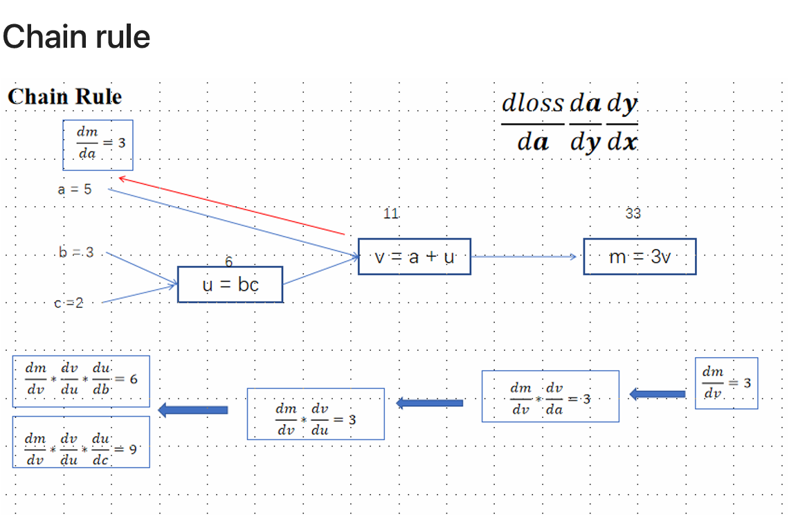
先写出关系公式，再求导。

---

三、反向传播：把误差“倒着传”回去

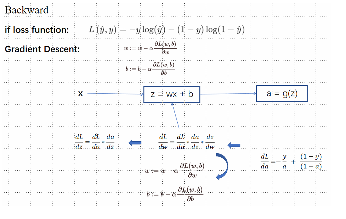
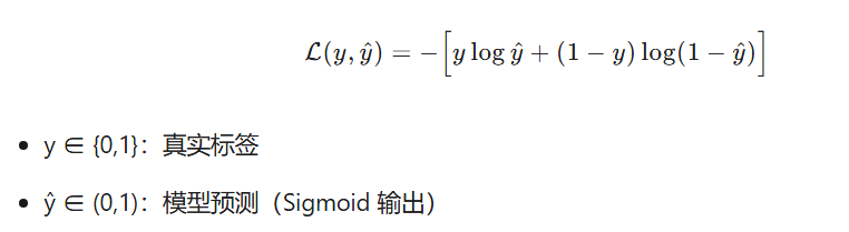
1. 流程图（文字版）

┌---------┐
│  输入X   │
└----┬----┘
     │前向
┌----┴----┐
│ 隐藏层Z¹ │←------┐
└----┬----┘       │
     │激活A¹      │梯度
┌----┴----┐       │
│ 输出层Z² │←------┘
└----┬----┘
     │激活A²
┌----┴----┐
│  损失L   │
└---------┘

2. 公式速查（不推导，直接记）

步骤	公式	维度说明
输出层误差	dZ² = A² − Y	(m,1)
输出层权重梯度	dW² = (A¹ᵀ · dZ²)/m	(hidden,1)
隐藏层误差	dZ¹ = (dZ² · W²ᵀ) ⊙ (1−A¹²)	(m,hidden)
隐藏层权重梯度	dW¹ = (Xᵀ · dZ¹)/m	(2,hidden)

⊙ 表示逐元素乘，m为样本数。

---

四、激活函数：为什么必须非线性？

若不用激活函数：

整个网络坍缩成单层线性模型，无法解决XOR等非线性问题。

常用非线性激活：

函数	公式	优点	缺点
Sigmoid	1/(1+e⁻ˣ)	平滑可导	易饱和、梯度消失
Tanh	(eˣ−e⁻ˣ)/(eˣ+e⁻ˣ)	零均值	同上
ReLU	max(0,x)	计算快、缓解梯度消失	“神经元死亡”
Leaky ReLU	max(0.01x,x)	解决死亡问题	多一个超参

---

五、从零实现神经网络

1.1 Import Required Packages - Generating Necessary Data

import numpy as np
# Import function to generate a moons dataset
from sklearn.datasets import make_moons  
# Import function to split dataset into training and test sets
from sklearn.model_selection import train_test_split 
# Import function to calculate accuracy score
from sklearn.metrics import accuracy_score  
import matplotlib.pyplot as plt
# Generate synthetic data
# Generate a 2D dataset with 1000 samples
X, y = make_moons(n_samples=1000, noise=0.2, random_state=42)
y = y.reshape(-1, 1) 
plt.hist(y)
plt.title("The value of Label Y and its quantity")
plt.xlabel("value")
plt.ylabel("quantity")
plt.show()
# Split into training and test sets
X_train, X_test, y_train, y_test = train_test_split(X, y, test_size=0.2, random_state=42)

1.2 Initialize the Model’s Parameters

① Here, we need to implement the function
initialize_parameters() .

② We must ensure our parameters’ sizes are appropriate.

③ We will initialize the weight matrix with random values.

def initialize_parameters(input_dim, hidden_dim, output_dim):
    np.random.seed(42)  # Set random seed for reproducibility
    # Initialize weights for the first layer
    W1 = np.random.randn(input_dim, hidden_dim) / np.sqrt(input_dim)  
    b1 = np.zeros((1, hidden_dim))  # Initialize biases for the first layer
    # Initialize weights for the second layer
    W2 = np.random.randn(hidden_dim, output_dim) / np.sqrt(hidden_dim)  
    b2 = np.zeros((1, output_dim))  # Initialize biases for the second layer
    return {"W1": W1, "b1": b1, "W2": W2, "b2": b2}  # Return initialized parameters

1.3 Activation Functions

def sigmoid(z):
    return 1 / (1 + np.exp(-z))

1.4 Forward Propagation

def forward_propagation(X, parameters):
    # Unpack parameters
    W1, b1, W2, b2 = parameters["W1"], parameters["b1"], parameters["W2"], parameters["b2"]
    # Compute first layer activations
    Z1 = np.dot(X, W1) + b1
    A1 = np.tanh(Z1)
    # Compute second layer activations
    Z2 = np.dot(A1, W2) + b2
    A2 = sigmoid(Z2)
    # Cache intermediate values for use in backpropagation
    cache = {"Z1": Z1, "A1": A1, "Z2": Z2, "A2": A2}  
    # Return activation value of the output layer and cached intermediate va
    return A2, cache 

1.5 Compute Loss

def compute_cost(A2, Y):
    m = Y.shape[0]  # Get number of samples
    # Compute cross-entropy loss
    logprobs = np.multiply(np.log(A2), Y) + np.multiply((1 - Y), np.log(1 - A2))
    cost = - np.sum(logprobs) / m  # Compute average loss over the dataset
    return cost  # Return cost

1.6 Backward Propagation

def backward_propagation(parameters, cache, X, Y):
    m = X.shape[0]  # Get number of samples
    A1 = cache["A1"]  # Retrieve activation values of the first layer from c
    A2 = cache["A2"]  # Retrieve activation values of the second layer from 
    dZ2 = A2 - Y  # Calculate gradient at output layer
    dW2 = np.dot(A1.T, dZ2) / m  # Calculate gradient of the loss with respe
    # Calculate gradient of the loss with respect to b2
    db2 = np.sum(dZ2, axis=0, keepdims=True) / m  
    dZ1 = np.dot(dZ2, parameters["W2"].T) * (1 - np.power(A1, 2))  # Calcula
    dW1 = np.dot(X.T, dZ1) / m  # Calculate gradient of the loss with respec
    # Calculate gradient ofS the loss with respect to b1
    db1 = np.sum(dZ1, axis=0, keepdims=True) / m  
    return {"dW1": dW1, "db1": db1, "dW2": dW2, "db2": db2}  # Return gradients

1.7 Update Parameters

 def update_parameters(parameters, grads, learning_rate=0.01):
    parameters["W1"] -= learning_rate * grads["dW1"]  # Update first layer w
    parameters["b1"] -= learning_rate * grads["db1"]  # Update first layer b
    parameters["W2"] -= learning_rate * grads["dW2"]  # Update second layer 
    parameters["b2"] -= learning_rate * grads["db2"]  # Update second layer 
    return parameters  # Return updated parameters

1.8 Batch Processing Data

# Batch generator for mini-batch gradient descent
 def batch_generator(X, Y, batch_size=32):
    indices = np.arange(X.shape[0])
    np.random.shuffle(indices)
    for start_idx in range(0, X.shape[0] - batch_size + 1, batch_size):
        excerpt = indices[start_idx:start_idx + batch_size]
        yield X[excerpt], Y[excerpt]

1.9 Model Training

 def model(X_train, Y_train, X_test, Y_test, n_hidden=4, n_epochs=20, batch_s
    np.random.seed(42)  # Seed random number generator
    n_input = X_train.shape[1]  # Determine input dimension
    n_output = Y_train.shape[1]  # Determine output dimension
    print(f'n_input = {n_input}, n_output = {n_output}')
    parameters = initialize_parameters(n_input, n_hidden, n_output)  # Initi
    for epoch in range(n_epochs):
        for X_batch, Y_batch in batch_generator(X_train, Y_train, batch_size
            A2, cache = forward_propagation(X_batch, parameters)  # Forward 
            cost = compute_cost(A2, Y_batch)  # Compute cost
            grads = backward_propagation(parameters, cache, X_batch, Y_batch
            parameters = update_parameters(parameters, grads)  # Update para
        
        if print_cost:
            print(f"Cost after epoch {epoch}: {cost}")
    
    return parameters  # Return learned parameters

1.10 Training the Model

parameters = model(X_train, y_train, X_test, y_test, n_hidden=4, n_epochs=10
print("W1 = " + str(parameters["W1"]))
print("b1 = " + str(parameters["b1"]))
print("W2 = " + str(parameters["W2"]))
print("b2 = " + str(parameters["b2"]))

1.11 Make Predictions

def predict(X_test, parameters):
    A2, _ = forward_propagation(X_test, parameters)  # Forward propagation w
    predictions = (A2 > 0.5)  # Convert probabilities to binary predictions
    accuracy = accuracy_score(y_test, predictions)  # Calculate accuracy on 
    print(f"Accuracy: {accuracy}")
    # TestingS
    # Prediction
predict(X_test, parameters)