【C++】哈希表详解 + unordered系列容器介绍与模拟实现
文章目录
上文链接
一、哈希表
哈希 (hash) 又称散列,是一种组织数据的方式。从译名来看,有散乱排列的意思。本质就是通过某种函数把关键字 key 跟它的存储位置建立一个映射关系,查找时通过这个函数计算出 key 存储的位置,进行快速查找。这种函数又叫做哈希函数。
比如,我想在一个数组中存储英文字母 a,a 的 ascii 码值为 97,那么我就可以把它存储在下标为 97 的位置上。这样一来我们存储的数据就和数组的下标就建立了一个映射关系,查找数据时就可以直接根据 ascii 码值来查找。
用上述方式存储数据的数据结构称为哈希表。
注:我们将关键字映射到数组中位置,一般是整数才好做映射计算,如果不是整数,我们要想办法转换成整数,这个细节我们后面代码实现中再进行细节展示。
二、哈希冲突
上述的映射关系存在的一个问题,那就是两个不同的 key 可能会映射到同一个位置去,这种问题我们叫做哈希冲突, 或者哈希碰撞。理想情况是找出一个好的哈希函数避免冲突,但是实际场景中,冲突是不可避免的, 所以我们尽可能设计出优秀的哈希函数,减少冲突的次数,同时也要去设计出解决冲突的方案。
那么如何合理地设计哈希函数,减少哈希冲突呢?下面提供几种方案。
三、哈希函数
1. 直接地址法
当关键字的范围比较集中时,直接定址法就是非常简单高效的方法。
-
比如一组关键字是在 [0,99] 之间的一些数字, 我们用哈希的思想存储这些数字只需要开一个大小为 100 的数组,每个关键字的值直接就是存储位置的下标;
-
再比如一组关键字是在 [a,z] 中的小写字母,那么我们只需开一个大小为 26 的数组,每个关键字
key存储在数组下标为key - 'a'的位置,这样我们查找某个字母时,就可以直接用该字母减去'a'到对应的下标处找即可。
也就是说直接定址法本质就是用关键字计算出一个绝对位置或者相对位置。
直接定址法的缺点也非常明显,当关键字的范围比较分散时,就很浪费内存甚至内存不够用。假设我们的数据为 [1, 2, 3, 9999],我们不可能去开一个 10000 大小的数组就为了存储这 4 个数字,这样就太浪费了。
2. 除法散列法
除法散列法也叫做除留余数法,顾名思义,假设哈希表的大小为
M
M
M,那么通过 key 除以
M
M
M 的余数就作为映射位置的下标,也就是哈希函数为
h
(
key
)
=
(key)
m
o
d
M
h(\operatorname{key})=\operatorname{(key)} \bmod M
h(key)=(key)modM
当使用除法散列时,要尽量避免
M
M
M 为某些值,如
2
2
2 的幂,
10
10
10 的幂等。
如果是 2 2 2 的幂 2 x 2^x 2x,那么 (key) m o d 2 x \operatorname{(key)} \bmod 2^x (key)mod2x 本质相当于保留 key 的后 x x x 位,也就是说后 x x x 位相同的数,计算出的哈希值都是一样的,就比较容易冲突。如:{63,31} 看起来没有关联的值,如果 M M M 是 16 16 16,那么计算出的哈希值都是 15 15 15,因为 63 63 63 的二进制后 8 位是 00111111, 31 31 31 的二进制后 8 位是 00011111。
如果是 10 10 10 的幂 1 0 x 10^x 10x,就更明显了,保留的都是 10 10 10 进值的后 x x x 位。如:{112,12312},如果 M M M 是 100 100 100,那么计算出的哈希值都是 12 12 12。
除此之外,建议 M M M 取不太接近 2 2 2 的整数次幂的一个质数 (素数)。
需要说明的是,实践中也是八仙过海,各显神通。Java 的 HashMap 采用除法散列法时就是
2
2
2 的整数次幂做哈希表的
M
M
M。这样玩的话,就不用取模,而是直接位运算,相对而言位运算比模更高效一些。比如
M
M
M 是
2
16
2^{16}
216 次方,本质是取后
16
16
16 位,那么用 key’ = key >> 16,然后把 key 和 key' 异或的结果作为哈希值,最终映射出的值还是在 [0,M) 范围内。只不过这样做是让 key 所有位都参与计算,哈希值会更均匀一些,减少冲突。所以我们上面建议
M
M
M 取不太接近
2
2
2 的整数次幂只是一个质数的理论,是大多数数据结构书籍中写的理论,但是实践中, 需要灵活运用,抓住本质。
3. 乘法散列法
乘法散列法对哈希表大小
M
M
M 没有要求,它的大思路就是用关键字 key 乘上一个常数
A
A
A
(
0
<
A
<
1
)
(0<A<1)
(0<A<1),并抽取出该乘积的小数部分,再用
M
M
M 乘以这个小数部分并向下取整,即
h
(
key
)
=
⌊
M
×
(
(
A
×
key
)
m
o
d
1.0
)
⌋
h(\operatorname{key}) = \lfloor M\times ((A\times \operatorname{key})\bmod 1.0)\rfloor
h(key)=⌊M×((A×key)mod1.0)⌋
这里最重要的是
A
A
A 的值应该如何设定,大佬 Knuth 认为
A
=
(
5
−
1
)
/
2
=
0.6180339887...
A=(\sqrt5 - 1) /2 = 0.6180339887...
A=(5−1)/2=0.6180339887... (黄金分割点) 比较好。
4. 全域散列法
如果存在一个恶意的对手,他针对我们提供的散列函数,特意构造出一个发生严重冲突的数据集,比如,让所有关键字全部落入同一个位置中。这种情况是可以存在的,只要散列函数是公开且确定的,就可以实现此攻击。解决方法自然是见招拆招,给散列函数增加随机性,攻击者就无法找出确定可以导致最坏情况的数据。这种方法叫做全域散列。比如
h
a
b
(
key
)
=
(
(
a
×
key
+
b
)
m
o
d
P
)
m
o
d
M
h_{ab}(\operatorname{key}) = ((a\times\operatorname{key} +\ b)\bmod P) \bmod M
hab(key)=((a×key+ b)modP)modM
P
P
P 需要选一个足够大的质数,
a
a
a 可以随机选一个
[
1
,
P
−
1
]
[1,P-1]
[1,P−1] 之间的整数,
b
b
b 可以随机选一个
[
0
,
P
−
1
]
[0,P-1]
[0,P−1] 之间的整数,这些函数共同构成了一个全域散列函数组。
需要注意的是每次初始化哈希表时,只需随机选取全域散列函数组中的一个散列函数使用,后续增删查改都固定使用这个散列函数,否则每次哈希都是随机选一个散列函数,那么插入是一个散列函数, 查找又是另一个散列函数,就会导致找不到插入的 key 了。
四、负载因子
假设哈希表中已经映射存储了 N N N 个值,哈希表的大小为 M M M,那么负载因子 = N M = \frac{N}{M} =MN。负载因子有些地方也翻译为载荷因子或装载因子等,它的英文为 loadfactor。负载因子越大,哈希冲突的概率越高,空间利用率越高;负载子越小,哈希冲突的概率越低,空间利用率越低。
五、处理哈希冲突
实践中哈希表一般还是选择除法散列法作为哈希函数,当然哈希表无论选择什么哈希函数也避免不了冲突,那么插入数据时,如何解决冲突呢?主要有两种两种方法,开放定址法和链地址法。
1. 开放地址法
在开放定址法中所有的元素都放到哈希表里,当一个关键字 key 用哈希函数计算出的位置冲突了,则按照某种规则找到一个没有存储数据的位置进行存储,开放定址法中负载因子一定是小于 1 的。这里的规则有三种:线性探测、二次探测、双重探测。
(1) 线性探测
从发生冲突的位置开始,依次线性向后探测,直到寻找到下一个没有存储数据的位置为止,如果走到哈希表尾,则回绕到哈希表头的位置。原本除留余数法的公式为
h
(
key
)
=
hash
0
=
(key)
m
o
d
M
h(\operatorname{key})= \operatorname{hash}0 = \operatorname{(key)} \bmod M
h(key)=hash0=(key)modM
如果
hash
0
\operatorname{hash}0
hash0 位置冲突了,则公式为
h
c
(
key
,
i
)
=
hash
i
=
(
hash0
+
i
)
m
o
d
M
hc(\operatorname{key}, i)= \operatorname{hash}i = (\operatorname{hash0 } + \ i) \bmod M
hc(key,i)=hashi=(hash0+ i)modM
其中
i
=
1
,
2
,
3
,
.
.
.
M
−
1
i = {1, 2,3,...M-1}
i=1,2,3,...M−1。因为负载因子小于 1,所以最多探测
M
−
1
M-1
M−1 次。
下面演示 [19, 30, 5, 36, 13, 20, 21, 12] 这组数映射到
M
=
11
M = 11
M=11 的表中:

h(19) = 8,h(30) = 8,h(5) = 5,h(36) = 3,h(13) = 2,h(20) = 9,h(21) = 10,h(12) = 1

线性探测的比较简单且容易实现,线性探测的问题假设,hash0 位置连续冲突,hash0,hash1,hash2 位置已经存储数据了,后续映射到 hash0,hash1,hash2,hash3 的值都会争夺 hash3 位置,这种现象叫做群集/堆积。下面的二次探测可以一定程度改善这个问题。
(2) 二次探测
从发生冲突的位置开始,依次左右按二次方跳跃式探测,直到寻找到下一个没有存储数据的位置为止,如果往右走到哈希表尾,则回绕到哈希表头的位置;如果往左走到哈希表头,则回绕到哈希表尾的位置。原本的除留余数法的公式为
h
(
key
)
=
hash
0
=
(key)
m
o
d
M
h(\operatorname{key})= \operatorname{hash}0 = \operatorname{(key)} \bmod M
h(key)=hash0=(key)modM
如果
hash
0
\operatorname{hash}0
hash0 位置冲突了,则公式为
h
c
(
key
,
i
)
=
hash
i
=
(
hash0
±
i
2
)
m
o
d
M
hc(\operatorname{key}, i)= \operatorname{hash}i = (\operatorname{hash0 } \pm \ i^2) \bmod M
hc(key,i)=hashi=(hash0± i2)modM
其中
i
=
1
,
2
,
3
,
.
.
.
M
2
i = {1, 2,3,...\frac{M}{2}}
i=1,2,3,...2M。二次探测当
hash
i
=
(
hash
0
−
i
2
)
m
o
d
M
\operatorname{hash}i = (\operatorname{hash}0 - i^2) \bmod M
hashi=(hash0−i2)modM 时,若
hash
i
<
0
\operatorname{hash}i < 0
hashi<0,需要 hashi += M。
下面演示 [19, 30, 52, 63, 11, 22] 这组数映射到
M
=
11
M = 11
M=11 的表中:

h(19) = 8, h(30) = 8, h(52) = 8, h(63) = 8, h(11) = 0, h(22) = 0

(3) 双重散列
第一个哈希函数计算出的值发生冲突,则使用第二个哈希函数计算出一个跟 key 相关的偏移量值,不断往后探测,直到寻找到下一个没有存储数据的位置为止。原本的除留余数法的公式为
h
(
key
)
=
hash
0
=
(key)
m
o
d
M
h(\operatorname{key})= \operatorname{hash}0 = \operatorname{(key)} \bmod M
h(key)=hash0=(key)modM
如果
hash
0
\operatorname{hash}0
hash0 位置冲突了,则公式为
h
c
(
key
,
i
)
=
hash
i
=
(
hash0
+
i
×
h
2
(
key
)
)
m
o
d
M
hc(\operatorname{key}, i)= \operatorname{hash}i = (\operatorname{hash0 } + \ i\times h_2(\operatorname{key})) \bmod M
hc(key,i)=hashi=(hash0+ i×h2(key))modM
其中
i
=
1
,
2
,
3
,
.
.
.
M
−
1
i = {1, 2,3,...M-1}
i=1,2,3,...M−1。要求
h
2
(
key
)
h_2(\operatorname{key})
h2(key) 和
M
M
M 互质,这里有两种取值方法:
- 当 M M M 为 2 2 2 的整数次幂时, h 2 ( key ) h_2(\operatorname{key}) h2(key) 从 [ 0 , M − 1 ] [0,\ M - 1] [0, M−1] 中任选一个奇数;
- 当 M M M 为质数时, h 2 ( key ) = ( key ) m o d ( M − 1 ) + 1 h_2(\operatorname{key}) = (\operatorname{key}) \bmod (M - 1) + 1 h2(key)=(key)mod(M−1)+1。
2. 开放地址法代码实现
// HashTable.h
#pragma once
#include<iostream>
#include<vector>

using namespace std;

namespace open_adress
{
    // 哈希表中每个位置数据的状态
    enum State
    {
        EXIST,  // 存在有效数据
        EMPTY,  // 该位置为空
        DELETE  // 该位置的数据原本存在但被删除
    };

    // 哈希表中的数据
    template<class K, class V>
    struct HashData
    {
        pair<K, V> _kv;
        State _state = EMPTY;
    };

    // 仿函数,将数据转换为整型,如果数据本身为整型,直接返回即可
    template<class K>
    struct HashFunc
    {
        size_t operator()(const K& key) const
        {
            return (size_t)key;
        }
    };

    // 实践中经常用到字符串,这里特化一个字符串转整型的仿函数
    template<>
    struct HashFunc<string>
    {
        size_t operator()(const string& key) const
        {
            size_t hash = 0;
            for (auto ch : key)
            {
                hash += ch;
                // 如果单纯将每个字符的 ascii 码相加效果不是很好
                // 可以采用边加边乘的方式,这种方式也是一种经典的算法
                hash *= 131;  // BKDRHash 算法
            }

            return hash;
        }
    };

    // 库中的写法
    // 在挑选出的质数中寻找第一个大于等于 n 的值,作为扩容后容器的大小
    inline unsigned long __stl_next_prime(unsigned long n)
    {
        // Note: assumes long is at least 32 bits.
        static const int __stl_num_primes = 28;
        static const unsigned long __stl_prime_list[__stl_num_primes] =
        {
            53, 97, 193, 389, 769,
            1543, 3079, 6151, 12289, 24593,
            49157, 98317, 196613, 393241, 786433,
            1572869, 3145739, 6291469, 12582917, 25165843,
            50331653, 100663319, 201326611, 402653189, 805306457,
            1610612741, 3221225473, 4294967291
        };
        const unsigned long* first = __stl_prime_list;
        const unsigned long* last = __stl_prime_list + __stl_num_primes;
        const unsigned long* pos = lower_bound(first, last, n);
        return pos == last ? *(last - 1) : *pos;
    }

    // 哈希表
    template<class K, class V, class Hash = HashFunc<K>>
    class HashTable
    {
    public:
        HashTable(size_t n = __stl_next_prime(0))
            :_tables(n)
            , _n(0)
        {}

        // 插入数据
        bool Insert(const pair<K, V>& kv)
        {
            if (Find(kv.first))
                return false;

            // 扩容: 负载因子 >= 0.7 就扩容
            // 扩容必须重新开空间然后拷贝数据,因为按照除留余数法的逻辑扩容后原本的数据在新空间的位置可能发生改变
            if ((double)_n / (double)_tables.size() >= 0.7)
            {
                // 创建一个新的哈希表比创建一个新的 vector 写起来更方便,因为我们可以复用 Insert
                HashTable<K, V> newht(__stl_next_prime(_tables.size() + 1));
                for (size_t i = 0; i < _tables.size(); i++)
                {
                    if (_tables[i]._state == EXIST)
                    {
                        newht.Insert(_tables[i]._kv);
                    }
                }

                _tables.swap(newht._tables);
            }

            Hash hs;
            size_t hash0 = hs(kv.first) % _tables.size();
            size_t hashi = hash0;
            size_t i = 1;

            // 线性探测
            while (_tables[hashi]._state == EXIST)
            {
                hashi = hash0 + i;
                i++;
                hashi %= _tables.size();
            }

            _tables[hashi]._kv = kv;
            _tables[hashi]._state = EXIST;
            ++_n;

            return true;
        }

        // 查找数据
        HashData<K, V>* Find(const K& key)
        {
            Hash hs;
            size_t hash0 = hs(key) % _tables.size();
            size_t hashi = hash0;
            size_t i = 1;

            while (_tables[hashi]._state != EMPTY)
            {
                if (_tables[hashi]._state == EXIST
                    && _tables[hashi]._kv.first == key)
                {
                    return &_tables[hashi];
                }

                hashi = hash0 + i;
                i++;
                hashi %= _tables.size();
            }

            return nullptr;
        }

        // 删除数据,不需要对数据本身做处理,只需把状态改为 DELETE 即可
        bool Erase(const K& key)
        {
            HashData<K, V>* ret = Find(key);
            if (ret)
            {
                ret->_state = DELETE;
                --_n;
                return true;
            }
            else
                return false;
        }

    private:
        vector<HashData<K, V>> _tables;
        size_t _n;  // 实际存储的数据个数
    };
}
3. 链地址法
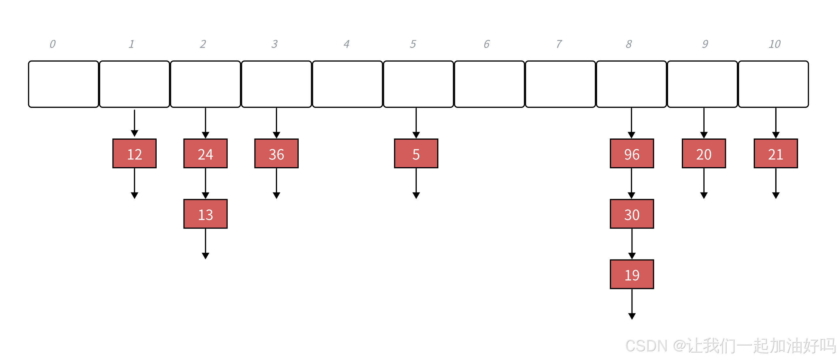
开放定址法中所有的元素都放到哈希表里,链地址法中所有的数据不再直接存储在哈希表中,哈希表中存储一个指针,没有数据映射这个位置时,这个指针为空,有多个数据映射到这个位置时,我们把这些冲突的数据链接成一个链表,挂在哈希表这个位置下面,链地址法也叫做拉链法或者哈希桶。
下面演示 19,30,5,36,13,20,21,12,24,96 这一组数映射到
M
=
11
M=11
M=11 的表中:

h(19) = 8,h(30) = 8,h(5) = 5,h(36) = 3,h(13) = 2,h(20) = 9,h(21) = 10,h(12) = 1,h(24) = 2,h(96) = 8
链表为单链表,在链表中新增值的插入方式为头插。
4. 链地址法代码实现
namespace hash_bucket
{
    // 节点
	template<class K, class V>
	struct HashNode
	{
		pair<K, V> _kv;
		HashNode<K, V>* _next;

		HashNode(const pair<K, V>& kv)
			:_kv(kv)
			, _next(nullptr)
		{}
	};

	// 仿函数
	template<class K>
	struct HashFunc
	{
		size_t operator()(const K& key) const
		{
			return (size_t)key;
		}
	};

	// 特化
	template<>
	struct HashFunc<string>
	{
		size_t operator()(const string& key) const
		{
			size_t hash = 0;
			for (auto ch : key)
			{
				hash += ch;
				hash *= 131;  // BKDRHash 算法
			}

			return hash;
		}
	};

    // 库中的写法
    // 在挑选出的质数中寻找第一个大于等于 n 的值,作为扩容后容器的大小
	inline unsigned long __stl_next_prime(unsigned long n)
	{
		// Note: assumes long is at least 32 bits.
		static const int __stl_num_primes = 28;
		static const unsigned long __stl_prime_list[__stl_num_primes] =
		{
			53, 97, 193, 389, 769,
			1543, 3079, 6151, 12289, 24593,
			49157, 98317, 196613, 393241, 786433,
			1572869, 3145739, 6291469, 12582917, 25165843,
			50331653, 100663319, 201326611, 402653189, 805306457,
			1610612741, 3221225473, 4294967291
		};
		const unsigned long* first = __stl_prime_list;
		const unsigned long* last = __stl_prime_list + __stl_num_primes;
		const unsigned long* pos = lower_bound(first, last, n);
		return pos == last ? *(last - 1) : *pos;
	}

	template<class K, class V, class Hash = HashFunc<K>>
	class HashTable
	{
		typedef HashNode<K, V> Node;
	public:
		HashTable(size_t n = __stl_next_prime(0))
			:_tables(n, nullptr)
			, _n(0)
		{}

		~HashTable()
		{
			for (size_t i = 0; i < _tables.size(); i++)
			{
				Node* cur = _tables[i];
				while (cur)
				{
					Node* next = cur->_next;
					delete cur;
					cur = next;
				}

				_tables[i] = nullptr;
			}
		}

		bool Insert(const pair<K, V>& kv)
		{
			if (Find(kv.first))
				return false;

			Hash hs;

			// 扩容: 负载因子到 1 时扩容
			if (_n == _tables.size())
			{
				//HashTable<K, V> newht(__stl_next_prime(_tables.size() + 1);

				//// 遍历旧表, 将旧表的数据全部重新映射到新表
				//for (size_t i = 0; i < _tables.size(); i++)
				//{
				//	Node* cur = _tables[i];
				//	while (cur)
				//	{
				//		newht.Insert(cur->_kv);
				//		cur = cur->_next;
				//	}
				//}

				// 上面这种方法需要创建节点和释放节点,有一定的消耗
				// 我们不妨直接移动旧的节点,这样就不用创建和释放了
				vector<Node*> newtables(__stl_next_prime(_tables.size() + 1), nullptr);

				// 遍历旧表, 将旧表的数据全部重新映射到新表
				for (size_t i = 0; i < _tables.size(); i++)
				{
					Node* cur = _tables[i];
					while (cur)
					{
						Node* next = cur->_next;
						// cur头插到新表
						size_t hashi = hs(cur->_kv.first) % newtables.size();
						cur->_next = newtables[hashi];
						newtables[hashi] = cur;

						cur = next;
					}
					// 移动完之后把旧表的数据置空
					_tables[i] = nullptr;
				}
				_tables.swap(newtables);
			}

			size_t hashi = hs(kv.first) % _tables.size();

			Node* newnode = new Node(kv);
			// 头插
			newnode->_next = _tables[hashi];
			_tables[hashi] = newnode;
			++_n;

			return true;
		}

		Node* Find(const K& key)
		{
			Hash hs;
			size_t hashi = hs(key) % _tables.size();
			Node* cur = _tables[hashi];
			while (cur)
			{
				if (cur->_kv.first == key)
					return cur;
				else
					cur = cur->_next;
			}
			return nullptr;
		}

		bool Erase(const K& key)
		{
			Hash hs;
			size_t hashi = hs(key) % _tables.size();
			Node* prev = nullptr;
			Node* cur = _tables[hashi];
			while (cur)
			{
				if (cur->_kv.first == key)
				{
					if (prev == nullptr)
						_tables[hashi] = cur->_next;
					else
						prev->_next = cur->_next;

					delete cur;
					--_n;
					return true;
				}
				else
				{
					prev = cur;
					cur = cur->_next;
				}
			}
			return false;
		}

	private:
		vector<Node*> _tables;
		size_t _n;  // 实际存储有效数据的个数
	};
}
六、STL 中的哈希表
1. unordered_set
unordered_set 是 STL 中的容器,它的增删查且跟 set 的使用一模一样,关于使用这里就不再赘述了,那么它们有什么区别呢?
-
unordered_set 底层是哈希表,增删查平均效率是 O ( 1 ) O(1) O(1);而 set 的底层是红黑树,增删查的效率为 O ( log N ) O(\operatorname{log}N) O(logN)。unordered_set 的迭代器遍历不再有序,为了跟 set 区分,所以取名为 unordered_set。
-
unordered_set 和 set 对 key 的要求不同,set 要求 key 支持小于比较,而 unordered_set 要求 key 支持转成整形且支持等于比较,本质其实是哈希表的要求。如果不支持则需要自己写仿函数。
-
unordered_set 和 set 的迭代器有差异,set 的 iterator 是双向迭代器,unordered_set 的则是单向迭代器。
2. unordered_map
unordered_map 与 map 的使用也是一模一样,它们的差异如下:
-
unordered_map 底层是哈希表,增删查平均效率是 O ( 1 ) O(1) O(1);而 map 的底层是红黑树,增删查的效率为 O ( log N ) O(\operatorname{log}N) O(logN)。
-
unordered_map 和 map 对 key 的要求不同,map 要求 key 支持小于比较,而 unordered_map 要求 key 支持转成整形且支持等于比较,本质是哈希表的要求。如果不支持则需要自己写仿函数。
-
unordered_map 和 map 的迭代器有差异,map 的 iterator 是双向迭代器, unordered_map 的则是单向迭代器。
七、封装哈希表实现 unordered_set 与 unordered_map
1. HashTable.h
#pragma once
#include<iostream>
#include<vector>
#include<algorithm>

using namespace std;

namespace hash_bucket
{
	template<class T>
	struct HashNode
	{
		T _data;
		HashNode<T>* _next;

		HashNode(const T& data)
			:_data(data)
			, _next(nullptr)
		{}
	};

	// 仿函数
	template<class K>
	struct HashFunc
	{
		size_t operator()(const K& key) const
		{
			return (size_t)key;
		}
	};

	// 特化
	template<>
	struct HashFunc<string>
	{
		size_t operator()(const string& key) const
		{
			size_t hash = 0;
			for (auto ch : key)
			{
				hash += ch;
				hash *= 131;  // BKDRHash 算法
			}

			return hash;
		}
	};

    // 库中的写法
    // 在挑选出的质数中寻找第一个大于等于 n 的值,作为扩容后容器的大小
	inline unsigned long __stl_next_prime(unsigned long n)
	{
		// Note: assumes long is at least 32 bits.
		static const int __stl_num_primes = 28;
		static const unsigned long __stl_prime_list[__stl_num_primes] =
		{
			53, 97, 193, 389, 769,
			1543, 3079, 6151, 12289, 24593,
			49157, 98317, 196613, 393241, 786433,
			1572869, 3145739, 6291469, 12582917, 25165843,
			50331653, 100663319, 201326611, 402653189, 805306457,
			1610612741, 3221225473, 4294967291
		};
		const unsigned long* first = __stl_prime_list;
		const unsigned long* last = __stl_prime_list + __stl_num_primes;
		const unsigned long* pos = lower_bound(first, last, n);
		return pos == last ? *(last - 1) : *pos;
	}

	// 前置声明, 因为 HTIterator 中用到了 HashTable, 而它的定义在后面, 所以防止编译器不认识, 就需要前置声明
	template<class K, class T, class KeyOfT, class Hash>
	class HashTable;

	template<class K, class T, class Ref, class Ptr, class KeyOfT, class Hash>
	struct HTIterator
	{
		typedef HashNode<T> Node;
		typedef HashTable<K, T, KeyOfT, Hash> HT;
		typedef HTIterator<K, T, Ref, Ptr, KeyOfT, Hash> Self;

		Node* _node;
		const HT* _pht;  // 这里加 const 是因为后面const迭代器要返回 ConstIterator(..., this), 而这里的 this 时是 const 对象必须要用 const 接收

		HTIterator(Node* node, const HT* pht)
			:_node(node)
			, _pht(pht)
		{}

		Ref operator*()
		{
			return _node->_data;
		}

		Ptr operator->()
		{
			return &_node->_data;
		}

		Self& operator++()
		{
			if (_node->_next)
			{
				// 当前桶还没有走完
				_node = _node->_next;
				return *this;
			}
			else
			{
				// 当前桶已经走完了, 需要找下一个不为空的桶里面的第一个节点
				KeyOfT kot;
				Hash hs;
				size_t hashi = hs(kot(_node->_data)) % _pht->_tables.size();
				hashi++;
				while (hashi < _pht->_tables.size())
				{
					if (_pht->_tables[hashi])
					{
						_node = _pht->_tables[hashi];
						break;
					}
					++hashi;
				}

				if (hashi == _pht->_tables.size())
				{
					// 所有桶都走完了, 就返回 end(), 这里 end() 就是空
					_node = nullptr;
				}

				return *this;
			}
		}

		bool operator!=(const Self& s) const
		{
			return _node != s._node;
		}

		bool operator==(const Self& s) const
		{
			return _node == s._node;
		}
	};

	template<class K, class T, class KeyOfT, class Hash>
	class HashTable
	{
		// 友元声明, 因为迭代器要访问哈希表的 _tables
		template<class K, class T, class Ref, class Ptr, class KeyOfT, class Hash>
		friend struct HTIterator;

		typedef HashNode<T> Node;
	public:
		typedef HTIterator<K, T, T&, T*, KeyOfT, Hash> Iterator;
		typedef HTIterator<K, T, const T&, const T*, KeyOfT, Hash> ConstIterator;

		Iterator Begin()
		{
			if (_n == 0)
				return End();

			for (size_t i = 0; i < _tables.size(); i++)
			{
				if (_tables[i])
					return Iterator(_tables[i], this);
			}

			return End();
		}

		Iterator End()
		{
			return Iterator(nullptr, this);
		}

		ConstIterator Begin() const
		{
			if (_n == 0)
				return End();

			for (size_t i = 0; i < _tables.size(); i++)
			{
				if (_tables[i])
					return ConstIterator(_tables[i], this);
			}

			return End();
		}

		ConstIterator End() const
		{
			return ConstIterator(nullptr, this);
		}

		HashTable(size_t n = __stl_next_prime(0))
			:_tables(n, nullptr)
			, _n(0)
		{}

		~HashTable()
		{
			for (size_t i = 0; i < _tables.size(); i++)
			{
				Node* cur = _tables[i];
				while (cur)
				{
					Node* next = cur->_next;
					delete cur;
					cur = next;
				}

				_tables[i] = nullptr;
			}
		}

		pair<Iterator, bool> Insert(const T& data)
		{
			KeyOfT kot;
			Iterator it = Find(kot(data));

			if (it != End())
				return { it, false };

			Hash hs;

			// 扩容: 负载因子到 1 时扩容
			if (_n == _tables.size())
			{
				//HashTable<K, V> newht(__stl_next_prime(_tables.size() + 1);

				//// 遍历旧表, 将旧表的数据全部重新映射到新表
				//for (size_t i = 0; i < _tables.size(); i++)
				//{
				//	Node* cur = _tables[i];
				//	while (cur)
				//	{
				//		newht.Insert(cur->_kv);
				//		cur = cur->_next;
				//	}
				//}

				// 上面这种方法需要创建节点和释放节点,有一定的消耗
				// 我们不妨直接移动旧的节点,这样就不用创建和释放了
				vector<Node*> newtables(__stl_next_prime(_tables.size() + 1), nullptr);

				// 遍历旧表, 将旧表的数据全部重新映射到新表
				for (size_t i = 0; i < _tables.size(); i++)
				{
					Node* cur = _tables[i];
					while (cur)
					{
						Node* next = cur->_next;
						// cur头插到新表
						size_t hashi = hs(kot(cur->_data)) % newtables.size();
						cur->_next = newtables[hashi];
						newtables[hashi] = cur;

						cur = next;
					}
					// 移动完之后把旧表的数据置空
					_tables[i] = nullptr;
				}
				_tables.swap(newtables);
			}

			size_t hashi = hs(kot(data)) % _tables.size();

			Node* newnode = new Node(data);
			// 头插
			newnode->_next = _tables[hashi];
			_tables[hashi] = newnode;
			++_n;

			return { Iterator(newnode, this), true };
		}

		Iterator Find(const K& key)
		{
			KeyOfT kot;
			Hash hs;
			size_t hashi = hs(key) % _tables.size();
			Node* cur = _tables[hashi];
			while (cur)
			{
				if (kot(cur->_data) == key)
					return Iterator(cur, this);
				else
					cur = cur->_next;
			}
			return End();
		}

		bool Erase(const K& key)
		{
			KeyOfT kot;
			Hash hs;
			size_t hashi = hs(key) % _tables.size();
			Node* prev = nullptr;
			Node* cur = _tables[hashi];
			while (cur)
			{
				if (kot(cur->_data) == key)
				{
					if (prev == nullptr)
						_tables[hashi] = cur->_next;
					else
						prev->_next = cur->_next;

					delete cur;
					--_n;
					return true;
				}
				else
				{
					prev = cur;
					cur = cur->_next;
				}
			}
			return false;
		}

	private:
		vector<Node*> _tables;
		size_t _n;  // 实际存储有效数据的个数
	};
}
2. myunordered_set.h
#pragma once

namespace mine
{
	template<class K, class Hash = hash_bucket::HashFunc<K>>
	class unordered_set
	{
		struct SetKeyOfT
		{
			const K& operator()(const K& key)
			{
				return key;
			}
		};

	public:
		typedef typename hash_bucket::HashTable<K, const K, SetKeyOfT, Hash>::Iterator iterator;
		typedef typename hash_bucket::HashTable<K, const K, SetKeyOfT, Hash>::ConstIterator const_iterator;

		iterator begin()
		{
			return _ht.Begin();
		}

		iterator end()
		{
			return _ht.End();
		}

		const_iterator begin() const
		{
			return _ht.Begin();
		}

		const_iterator end() const
		{
			return _ht.End();
		}

		pair<iterator, bool> insert(const K& key)
		{
			return _ht.Insert(key);
		}

		iterator find(const K& key)
		{
			return _ht.Find(key);
		}

		bool erase(const K& key)
		{
			return _ht.erase(key);
		}

	private:
		hash_bucket::HashTable<K, const K, SetKeyOfT, Hash> _ht;
	};
}
3. myunordered_map.h
#pragma once

namespace mine
{
	template<class K, class V, class Hash = hash_bucket::HashFunc<K>>
	class unordered_map
	{
		struct MapKeyOfT
		{
			const K& operator()(const pair<K, V>& kv)
			{
				return kv.first;
			}
		};

	public:
		typedef typename hash_bucket::HashTable<K, pair<const K, V>, MapKeyOfT, Hash>::Iterator iterator;
		typedef typename hash_bucket::HashTable<K, pair<const K, V>, MapKeyOfT, Hash>::ConstIterator const_iterator;

		iterator begin()
		{
			return _ht.Begin();
		}

		iterator end()
		{
			return _ht.End();
		}

		const_iterator begin() const
		{
			return _ht.Begin();
		}

		const_iterator end() const
		{
			return _ht.End();
		}

		pair<iterator, bool> insert(const pair<K, V>& kv)
		{
			return _ht.Insert(kv);
		}

		iterator find(const K& key)
		{
			return _ht.Find(key);
		}

		bool erase(const K& key)
		{
			return _ht.erase(key);
		}

		V& operator[](const K& key)
		{
			pair<iterator, bool> ret = insert({ key, V() });
			return ret.first->second;
		}

	private:
		hash_bucket::HashTable<K, pair<const K, V>, MapKeyOfT, Hash> _ht;
	};
}
下文链接

码道开发者社区,聚焦华为云码道 CodeArts 代码智能体,沉淀 Agent、Skill、鸿蒙开发实战内容,供开发者查阅资料、交流技术、分享工程实践
更多推荐



 14
14 0
0- 0


 已为社区贡献1条内容

所有评论(0)